

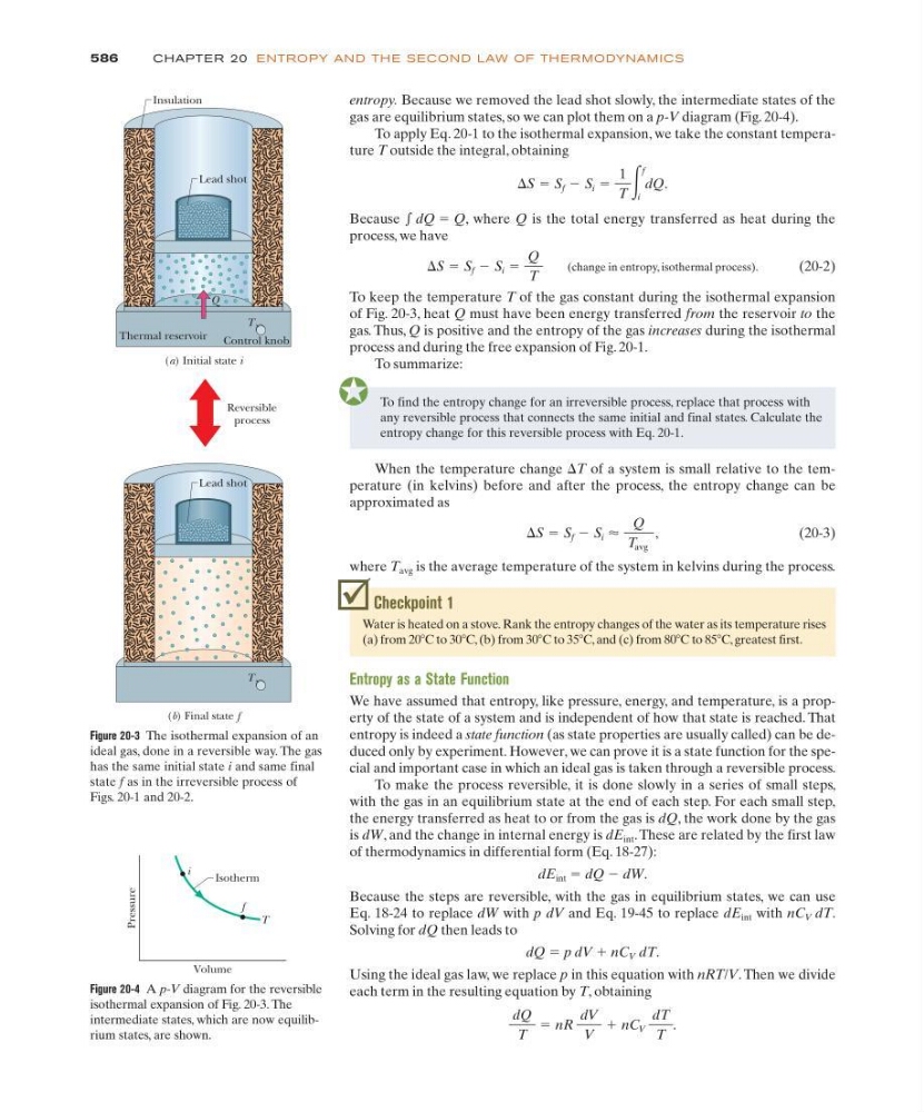
entropy. Because we removed the lead shot slowly, the intermediate states of the
gas are equilibrium states, so we can plot them on a p-V diagram (Fig. 20-4).
To apply Eq. 20-1 to the isothermal expansion, we take the constant temperature T outside the integral, obtaining
Because ͐ dQ ϭ Q, where Q is the total energy transferred as heat during the
process, we have
(change in entropy, isothermal process).
(20-2)
To keep the temperature T of the gas constant during the isothermal expansion
of Fig. 20-3, heat Q must have been energy transferred from the reservoir to the
gas. Thus, Q is positive and the entropy of the gas increases during the isothermal
process and during the free expansion of Fig. 20-1.
To summarize:
⌬S ϭ S f Ϫ S i ϭ
Q
T
⌬S ϭ S f Ϫ S i ϭ
1
T
͵
f
i
dQ.
586
CHAPTE R 20 ENTROPY AND THE SECOND LAW OF THERMODYNAM ICS
T
Lead shot
Insulation
Thermal reservoir
T
Control knob
Q
(a) Initial state i
Reversible
process
Lead shot
(b) Final state f
Figure 20-3 The isothermal expansion of an
ideal gas, done in a reversible way. The gas
has the same initial state i and same final
state f as in the irreversible process of
Figs. 20-1 and 20-2.
Figure 20-4 A p-V diagram for the reversible
isothermal expansion of Fig. 20-3. The
intermediate states, which are now equilibrium states, are shown.
Isotherm
T
Pressure
Volume
i
f
To find the entropy change for an irreversible process, replace that process with
any reversible process that connects the same initial and final states. Calculate the
entropy change for this reversible process with Eq. 20-1.
When the temperature change ⌬T of a system is small relative to the temperature (in kelvins) before and after the process, the entropy change can be
approximated as
(20-3)
where T avg is the average temperature of the system in kelvins during the process.
⌬S ϭ S f Ϫ S i Ϸ
Q
T avg
,
Checkpoint 1
Water is heated on a stove. Rank the entropy changes of the water as its temperature rises
(a) from 20ЊC to 30ЊC, (b) from 30ЊC to 35ЊC, and (c) from 80ЊC to 85ЊC, greatest first.
Entropy as a State Function
We have assumed that entropy, like pressure, energy, and temperature, is a property of the state of a system and is independent of how that state is reached. That
entropy is indeed a state function (as state properties are usually called) can be deduced only by experiment. However, we can prove it is a state function for the special and important case in which an ideal gas is taken through a reversible process.
To make the process reversible, it is done slowly in a series of small steps,
with the gas in an equilibrium state at the end of each step. For each small step,
the energy transferred as heat to or from the gas is dQ, the work done by the gas
is dW, and the change in internal energy is dE int . These are related by the first law
of thermodynamics in differential form (Eq. 18-27):
dE int ϭ dQ Ϫ dW.
Because the steps are reversible, with the gas in equilibrium states, we can use
Eq. 18-24 to replace dW with p dV and Eq. 19-45 to replace dE int with nC V dT.
Solving for dQ then leads to
dQ ϭ p dV ϩ nC V dT.
Using the ideal gas law, we replace p in this equation with nRT/V. Then we divide
each term in the resulting equation by T, obtaining
dQ
T
ϭ nR
dV
V
ϩ nC V
dT
T
.
gas are equilibrium states, so we can plot them on a p-V diagram (Fig. 20-4).
To apply Eq. 20-1 to the isothermal expansion, we take the constant temperature T outside the integral, obtaining
Because ͐ dQ ϭ Q, where Q is the total energy transferred as heat during the
process, we have
(change in entropy, isothermal process).
(20-2)
To keep the temperature T of the gas constant during the isothermal expansion
of Fig. 20-3, heat Q must have been energy transferred from the reservoir to the
gas. Thus, Q is positive and the entropy of the gas increases during the isothermal
process and during the free expansion of Fig. 20-1.
To summarize:
⌬S ϭ S f Ϫ S i ϭ
Q
T
⌬S ϭ S f Ϫ S i ϭ
1
T
͵
f
i
dQ.
586
CHAPTE R 20 ENTROPY AND THE SECOND LAW OF THERMODYNAM ICS
T
Lead shot
Insulation
Thermal reservoir
T
Control knob
Q
(a) Initial state i
Reversible
process
Lead shot
(b) Final state f
Figure 20-3 The isothermal expansion of an
ideal gas, done in a reversible way. The gas
has the same initial state i and same final
state f as in the irreversible process of
Figs. 20-1 and 20-2.
Figure 20-4 A p-V diagram for the reversible
isothermal expansion of Fig. 20-3. The
intermediate states, which are now equilibrium states, are shown.
Isotherm
T
Pressure
Volume
i
f
To find the entropy change for an irreversible process, replace that process with
any reversible process that connects the same initial and final states. Calculate the
entropy change for this reversible process with Eq. 20-1.
When the temperature change ⌬T of a system is small relative to the temperature (in kelvins) before and after the process, the entropy change can be
approximated as
(20-3)
where T avg is the average temperature of the system in kelvins during the process.
⌬S ϭ S f Ϫ S i Ϸ
Q
T avg
,
Checkpoint 1
Water is heated on a stove. Rank the entropy changes of the water as its temperature rises
(a) from 20ЊC to 30ЊC, (b) from 30ЊC to 35ЊC, and (c) from 80ЊC to 85ЊC, greatest first.
Entropy as a State Function
We have assumed that entropy, like pressure, energy, and temperature, is a property of the state of a system and is independent of how that state is reached. That
entropy is indeed a state function (as state properties are usually called) can be deduced only by experiment. However, we can prove it is a state function for the special and important case in which an ideal gas is taken through a reversible process.
To make the process reversible, it is done slowly in a series of small steps,
with the gas in an equilibrium state at the end of each step. For each small step,
the energy transferred as heat to or from the gas is dQ, the work done by the gas
is dW, and the change in internal energy is dE int . These are related by the first law
of thermodynamics in differential form (Eq. 18-27):
dE int ϭ dQ Ϫ dW.
Because the steps are reversible, with the gas in equilibrium states, we can use
Eq. 18-24 to replace dW with p dV and Eq. 19-45 to replace dE int with nC V dT.
Solving for dQ then leads to
dQ ϭ p dV ϩ nC V dT.
Using the ideal gas law, we replace p in this equation with nRT/V. Then we divide
each term in the resulting equation by T, obtaining
dQ
T
ϭ nR
dV
V
ϩ nC V
dT
T
.