

29
2-6 GRAPHICAL INTEGRATION IN MOTION ANALYSIS
2-6 GRAPHICAL INTEGRATION IN MOTION ANALYSIS
After reading this module, you should be able to . . .
2.18 Determine a particle’s change in velocity by graphical
integration on a graph of acceleration versus time.
2.19 Determine a particle’s change in position by graphical
integration on a graph of velocity versus time.
● On a graph of acceleration a versus time t, the change in
the velocity is given by
The integral amounts to finding an area on the graph:
͵
t 1
t 0
a dt ϭ
area between acceleration curve
and time axis, from t 0 to t 1 .
v 1 Ϫ v 0 ϭ ͵
t 1
t 0
a dt.
● On a graph of velocity v versus time t, the change in the
position is given by
where the integral can be taken from the graph as
͵
t 1
t 0
v dt ϭ
area between velocity curve
and time axis, from t 0 to t 1
.
x 1 Ϫ x 0 ϭ ͵
t 1
t 0
v dt,
Learning Objectives
Key Ideas
Graphical Integration in Motion Analysis
Integrating Acceleration. When we have a graph of an object’s acceleration a versus time t, we can integrate on the graph to find the velocity at any given time.
Because a is defined as a ϭ dv/dt, the Fundamental Theorem of Calculus tells us that
(2-27)
The right side of the equation is a definite integral (it gives a numerical result rather
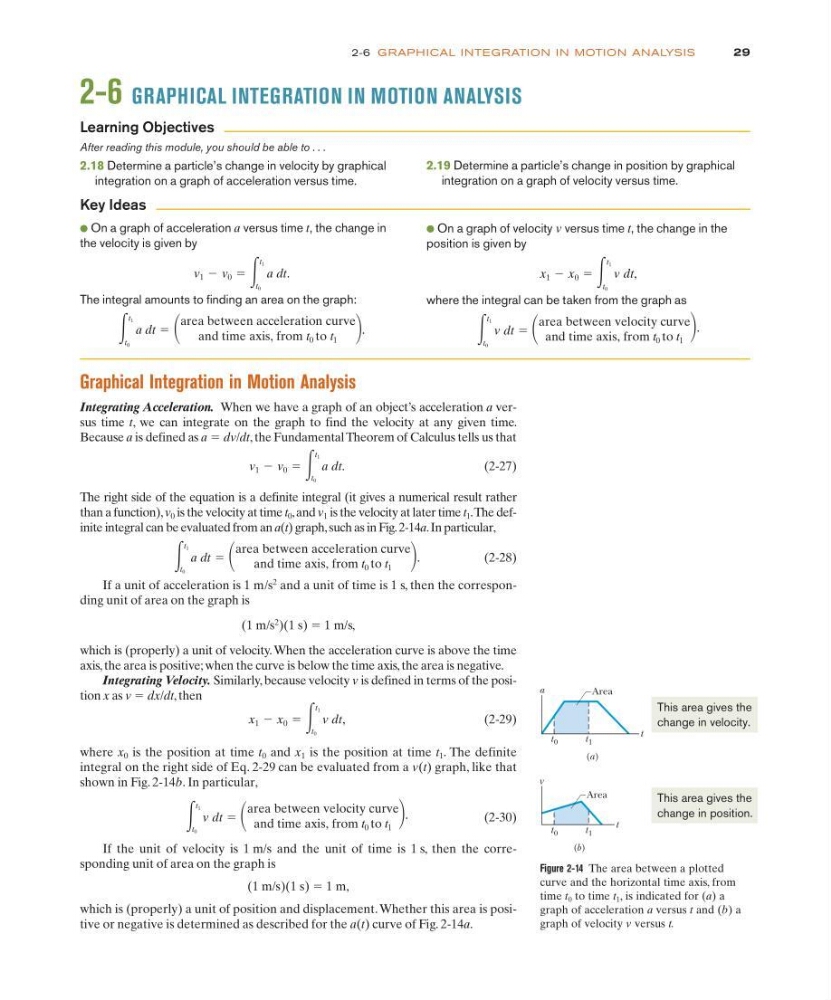
than a function), v 0 is the velocity at time t 0 ,and v 1 is the velocity at later time t 1 .The definite integral can be evaluated from an a(t) graph, such as in Fig. 2-14a.In particular,
(2-28)
If a unit of acceleration is 1 m/s
2
and a unit of time is 1 s, then the corresponding unit of area on the graph is
(1 m/s
2
)(1 s) ϭ 1 m/s,
which is (properly) a unit of velocity. When the acceleration curve is above the time
axis, the area is positive; when the curve is below the time axis, the area is negative.
Integrating Velocity. Similarly, because velocity v is defined in terms of the position x as v ϭ dx/dt, then
(2-29)
where x 0 is the position at time t 0 and x 1 is the position at time t 1 . The definite
integral on the right side of Eq. 2-29 can be evaluated from a v(t) graph, like that
shown in Fig. 2-14b. In particular,
(2-30)
If the unit of velocity is 1 m/s and the unit of time is 1 s, then the corresponding unit of area on the graph is
(1 m/s)(1 s) ϭ 1 m,
which is (properly) a unit of position and displacement. Whether this area is positive or negative is determined as described for the a(t) curve of Fig. 2-14a.
͵
t 1
t 0
v dt ϭ
area between velocity curve
and time axis, from t 0 to t 1
.
x 1 Ϫ x 0 ϭ ͵
t 1
t 0
v dt,
͵
t 1
t 0
a dt ϭ
area between acceleration curve
and time axis, from t 0 to t 1 .
v 1 Ϫ v 0 ϭ ͵
t 1
t 0
a dt.
Figure 2-14 The area between a plotted
curve and the horizontal time axis, from
time t 0 to time t 1 , is indicated for (a) a
graph of acceleration a versus t and (b) a
graph of velocity v versus t.
a
t 0
t
t 1
Area
(a)
v
t 0
t
t 1
Area
(b)
This area gives the
change in velocity.
This area gives the
change in position.
2-6 GRAPHICAL INTEGRATION IN MOTION ANALYSIS
2-6 GRAPHICAL INTEGRATION IN MOTION ANALYSIS
After reading this module, you should be able to . . .
2.18 Determine a particle’s change in velocity by graphical
integration on a graph of acceleration versus time.
2.19 Determine a particle’s change in position by graphical
integration on a graph of velocity versus time.
● On a graph of acceleration a versus time t, the change in
the velocity is given by
The integral amounts to finding an area on the graph:
͵
t 1
t 0
a dt ϭ
area between acceleration curve
and time axis, from t 0 to t 1 .
v 1 Ϫ v 0 ϭ ͵
t 1
t 0
a dt.
● On a graph of velocity v versus time t, the change in the
position is given by
where the integral can be taken from the graph as
͵
t 1
t 0
v dt ϭ
area between velocity curve
and time axis, from t 0 to t 1
.
x 1 Ϫ x 0 ϭ ͵
t 1
t 0
v dt,
Learning Objectives
Key Ideas
Graphical Integration in Motion Analysis
Integrating Acceleration. When we have a graph of an object’s acceleration a versus time t, we can integrate on the graph to find the velocity at any given time.
Because a is defined as a ϭ dv/dt, the Fundamental Theorem of Calculus tells us that
(2-27)
The right side of the equation is a definite integral (it gives a numerical result rather
than a function), v 0 is the velocity at time t 0 ,and v 1 is the velocity at later time t 1 .The definite integral can be evaluated from an a(t) graph, such as in Fig. 2-14a.In particular,
(2-28)
If a unit of acceleration is 1 m/s
2
and a unit of time is 1 s, then the corresponding unit of area on the graph is
(1 m/s
2
)(1 s) ϭ 1 m/s,
which is (properly) a unit of velocity. When the acceleration curve is above the time
axis, the area is positive; when the curve is below the time axis, the area is negative.
Integrating Velocity. Similarly, because velocity v is defined in terms of the position x as v ϭ dx/dt, then
(2-29)
where x 0 is the position at time t 0 and x 1 is the position at time t 1 . The definite
integral on the right side of Eq. 2-29 can be evaluated from a v(t) graph, like that
shown in Fig. 2-14b. In particular,
(2-30)
If the unit of velocity is 1 m/s and the unit of time is 1 s, then the corresponding unit of area on the graph is
(1 m/s)(1 s) ϭ 1 m,
which is (properly) a unit of position and displacement. Whether this area is positive or negative is determined as described for the a(t) curve of Fig. 2-14a.
͵
t 1
t 0
v dt ϭ
area between velocity curve
and time axis, from t 0 to t 1
.
x 1 Ϫ x 0 ϭ ͵
t 1
t 0
v dt,
͵
t 1
t 0
a dt ϭ
area between acceleration curve
and time axis, from t 0 to t 1 .
v 1 Ϫ v 0 ϭ ͵
t 1
t 0
a dt.
Figure 2-14 The area between a plotted
curve and the horizontal time axis, from
time t 0 to time t 1 , is indicated for (a) a
graph of acceleration a versus t and (b) a
graph of velocity v versus t.
a
t 0
t
t 1
Area
(a)
v
t 0
t
t 1
Area
(b)
This area gives the
change in velocity.
This area gives the
change in position.