

450
CHAPTE R 16 WAVES—I
Consider now a wave of arbitrary shape, given by
y(x, t) ϭ h(kx Ϯ vt),
(16-17)
where h represents any function, the sine function being one possibility. Our
previous analysis shows that all waves in which the variables x and t enter
into the combination kx Ϯ vt are traveling waves. Furthermore, all traveling
waves must be of the form of Eq. 16-17. Thus, y(x, t) ϭ
represents a
possible (though perhaps physically a little bizarre) traveling wave. The function
y(x, t) ϭ sin(ax
2 Ϫ bt), on the other hand, does not represent a traveling wave.
1ax ϩ bt
Checkpoint 2
Here are the equations of three waves:
(1) y(x, t) ϭ 2 sin(4x Ϫ 2t), (2) y(x, t) ϭ sin(3x Ϫ 4t), (3) y(x, t) ϭ 2 sin(3x Ϫ 3t).
Rank the waves according to their (a) wave speed and (b) maximum speed perpendicular to the wave’s direction of travel (the transverse speed), greatest first.
straction, showing us motion spread out over time. From it
we can determine the period T of the string element in its
SHM and thus also of the wave itself. From T we can then
find angular frequency v (ϭ 2p/T) in Eq. 16-18. (3) The
phase constant f is set by the displacement of the string at
x ϭ 0 and t ϭ 0.
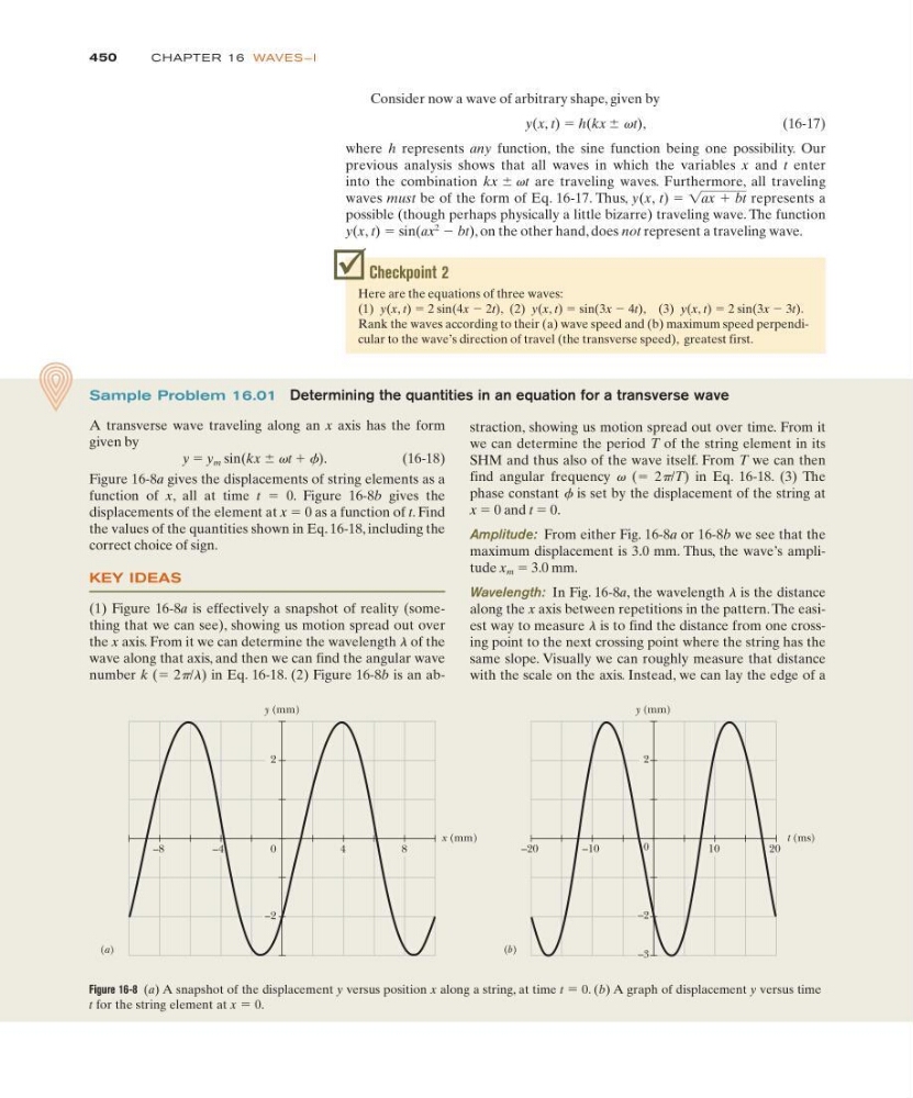
Amplitude: From either Fig. 16-8a or 16-8b we see that the
maximum displacement is 3.0 mm. Thus, the wave’s amplitude x m ϭ 3.0 mm.
Wavelength: In Fig. 16-8a, the wavelength l is the distance
along the x axis between repetitions in the pattern. The easiest way to measure l is to find the distance from one crossing point to the next crossing point where the string has the
same slope. Visually we can roughly measure that distance
with the scale on the axis. Instead, we can lay the edge of a
Sample Problem 16.01 Determining the quantities in an equation for a transverse wave
A transverse wave traveling along an x axis has the form
given by
y ϭ y m sin(kx Ϯ vt ϩ f).
(16-18)
Figure 16-8a gives the displacements of string elements as a
function of x, all at time t ϭ 0. Figure 16-8b gives the
displacements of the element at x ϭ 0 as a function of t. Find
the values of the quantities shown in Eq. 16-18, including the
correct choice of sign.
KEY IDEAS
(1) Figure 16-8a is effectively a snapshot of reality (something that we can see), showing us motion spread out over
the x axis. From it we can determine the wavelength l of the
wave along that axis, and then we can find the angular wave
number k (ϭ 2p/l) in Eq. 16-18. (2) Figure 16-8b is an abFigure 16-8 (a) A snapshot of the displacement y versus position x along a string, at time t ϭ 0. (b) A graph of displacement y versus time
t for the string element at x ϭ 0.
(a)
–8
2
–2
0
y (mm)
x (mm)
–4
4
8
(b)
0
y (mm)
t (ms)
–20
10
20
–10
–3
–2
2
CHAPTE R 16 WAVES—I
Consider now a wave of arbitrary shape, given by
y(x, t) ϭ h(kx Ϯ vt),
(16-17)
where h represents any function, the sine function being one possibility. Our
previous analysis shows that all waves in which the variables x and t enter
into the combination kx Ϯ vt are traveling waves. Furthermore, all traveling
waves must be of the form of Eq. 16-17. Thus, y(x, t) ϭ
represents a
possible (though perhaps physically a little bizarre) traveling wave. The function
y(x, t) ϭ sin(ax
2 Ϫ bt), on the other hand, does not represent a traveling wave.
1ax ϩ bt
Checkpoint 2
Here are the equations of three waves:
(1) y(x, t) ϭ 2 sin(4x Ϫ 2t), (2) y(x, t) ϭ sin(3x Ϫ 4t), (3) y(x, t) ϭ 2 sin(3x Ϫ 3t).
Rank the waves according to their (a) wave speed and (b) maximum speed perpendicular to the wave’s direction of travel (the transverse speed), greatest first.
straction, showing us motion spread out over time. From it
we can determine the period T of the string element in its
SHM and thus also of the wave itself. From T we can then
find angular frequency v (ϭ 2p/T) in Eq. 16-18. (3) The
phase constant f is set by the displacement of the string at
x ϭ 0 and t ϭ 0.
Amplitude: From either Fig. 16-8a or 16-8b we see that the
maximum displacement is 3.0 mm. Thus, the wave’s amplitude x m ϭ 3.0 mm.
Wavelength: In Fig. 16-8a, the wavelength l is the distance
along the x axis between repetitions in the pattern. The easiest way to measure l is to find the distance from one crossing point to the next crossing point where the string has the
same slope. Visually we can roughly measure that distance
with the scale on the axis. Instead, we can lay the edge of a
Sample Problem 16.01 Determining the quantities in an equation for a transverse wave
A transverse wave traveling along an x axis has the form
given by
y ϭ y m sin(kx Ϯ vt ϩ f).
(16-18)
Figure 16-8a gives the displacements of string elements as a
function of x, all at time t ϭ 0. Figure 16-8b gives the
displacements of the element at x ϭ 0 as a function of t. Find
the values of the quantities shown in Eq. 16-18, including the
correct choice of sign.
KEY IDEAS
(1) Figure 16-8a is effectively a snapshot of reality (something that we can see), showing us motion spread out over
the x axis. From it we can determine the wavelength l of the
wave along that axis, and then we can find the angular wave
number k (ϭ 2p/l) in Eq. 16-18. (2) Figure 16-8b is an abFigure 16-8 (a) A snapshot of the displacement y versus position x along a string, at time t ϭ 0. (b) A graph of displacement y versus time
t for the string element at x ϭ 0.
(a)
–8
2
–2
0
y (mm)
x (mm)
–4
4
8
(b)
0
y (mm)
t (ms)
–20
10
20
–10
–3
–2
2