

19
2-2 INSTANTANEOUS VELOCITY AND SPEED
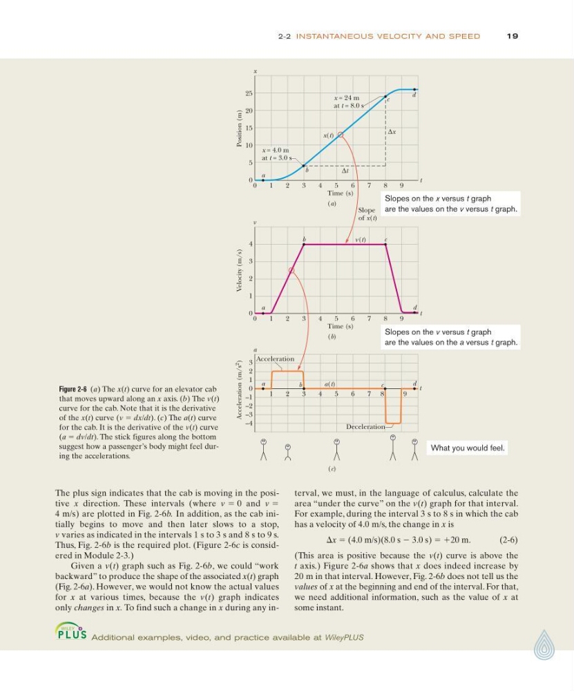
Figure 2-6 (a) The x(t) curve for an elevator cab
that moves upward along an x axis. (b) The v(t)
curve for the cab. Note that it is the derivative
of the x(t) curve (v ϭ dx/dt). (c) The a(t) curve
for the cab. It is the derivative of the v(t) curve
(a ϭ dv/dt). The stick figures along the bottom
suggest how a passenger’s body might feel during the accelerations.
Additional examples, video, and practice available at WileyPLUS
The plus sign indicates that the cab is moving in the positive x direction. These intervals (where v ϭ 0 and v ϭ
4 m/s) are plotted in Fig. 2-6b. In addition, as the cab initially begins to move and then later slows to a stop,
v varies as indicated in the intervals 1 s to 3 s and 8 s to 9 s.
Thus, Fig. 2-6b is the required plot. (Figure 2-6c is considered in Module 2-3.)
Given a v(t) graph such as Fig. 2-6b, we could “work
backward” to produce the shape of the associated x(t) graph
(Fig. 2-6a). However, we would not know the actual values
for x at various times, because the v(t) graph indicates
only changes in x. To find such a change in x during any inDeceleration
Position (m)
Time (s)
t
0
9
8
7
6
5
4
3
2
1
0
5
10
15
20
25
Slope
of x(t)
∆t
∆x
Velocity (m/s)
Time (s)
9
0
1
2
3
4
x
a
b
c
d
0
x(t)
v(t)
b
c
d
a
v
t
0
–1
–2
–3
–4
1
2
t
Acceleration (m/s
2
)
(a)
(b)
(c)
9
8
7
6
5
4
3
2
1
8
7
6
5
4
3
2
1
a
a(t)
Acceleration
c
b
a
d
3
x = 24 m
at t = 8.0 s
x = 4.0 m
at t = 3.0 s
Slopes on the x versus t graph
are the values on the v versus t graph.
Slopes on the v versus t graph
are the values on the a versus t graph.
What you would feel.
terval, we must, in the language of calculus, calculate the
area “under the curve” on the v(t) graph for that interval.
For example, during the interval 3 s to 8 s in which the cab
has a velocity of 4.0 m/s, the change in x is
⌬x ϭ (4.0 m/s)(8.0 s Ϫ 3.0 s) ϭ ϩ20 m.
(2-6)
(This area is positive because the v(t) curve is above the
t axis.) Figure 2-6a shows that x does indeed increase by
20 m in that interval. However, Fig. 2-6b does not tell us the
values of x at the beginning and end of the interval. For that,
we need additional information, such as the value of x at
some instant.
2-2 INSTANTANEOUS VELOCITY AND SPEED
Figure 2-6 (a) The x(t) curve for an elevator cab
that moves upward along an x axis. (b) The v(t)
curve for the cab. Note that it is the derivative
of the x(t) curve (v ϭ dx/dt). (c) The a(t) curve
for the cab. It is the derivative of the v(t) curve
(a ϭ dv/dt). The stick figures along the bottom
suggest how a passenger’s body might feel during the accelerations.
Additional examples, video, and practice available at WileyPLUS
The plus sign indicates that the cab is moving in the positive x direction. These intervals (where v ϭ 0 and v ϭ
4 m/s) are plotted in Fig. 2-6b. In addition, as the cab initially begins to move and then later slows to a stop,
v varies as indicated in the intervals 1 s to 3 s and 8 s to 9 s.
Thus, Fig. 2-6b is the required plot. (Figure 2-6c is considered in Module 2-3.)
Given a v(t) graph such as Fig. 2-6b, we could “work
backward” to produce the shape of the associated x(t) graph
(Fig. 2-6a). However, we would not know the actual values
for x at various times, because the v(t) graph indicates
only changes in x. To find such a change in x during any inDeceleration
Position (m)
Time (s)
t
0
9
8
7
6
5
4
3
2
1
0
5
10
15
20
25
Slope
of x(t)
∆t
∆x
Velocity (m/s)
Time (s)
9
0
1
2
3
4
x
a
b
c
d
0
x(t)
v(t)
b
c
d
a
v
t
0
–1
–2
–3
–4
1
2
t
Acceleration (m/s
2
)
(a)
(b)
(c)
9
8
7
6
5
4
3
2
1
8
7
6
5
4
3
2
1
a
a(t)
Acceleration
c
b
a
d
3
x = 24 m
at t = 8.0 s
x = 4.0 m
at t = 3.0 s
Slopes on the x versus t graph
are the values on the v versus t graph.
Slopes on the v versus t graph
are the values on the a versus t graph.
What you would feel.
terval, we must, in the language of calculus, calculate the
area “under the curve” on the v(t) graph for that interval.
For example, during the interval 3 s to 8 s in which the cab
has a velocity of 4.0 m/s, the change in x is
⌬x ϭ (4.0 m/s)(8.0 s Ϫ 3.0 s) ϭ ϩ20 m.
(2-6)
(This area is positive because the v(t) curve is above the
t axis.) Figure 2-6a shows that x does indeed increase by
20 m in that interval. However, Fig. 2-6b does not tell us the
values of x at the beginning and end of the interval. For that,
we need additional information, such as the value of x at
some instant.