

Displacement is an example of a vector quantity, which is a quantity that has
both a direction and a magnitude. We explore vectors more fully in Chapter 3, but
here all we need is the idea that displacement has two features: (1) Its magnitude
is the distance (such as the number of meters) between the original and final positions. (2) Its direction, from an original position to a final position, can be represented by a plus sign or a minus sign if the motion is along a single axis.
Here is the first of many checkpoints where you can check your understanding
with a bit of reasoning. The answers are in the back of the book.
15
2-1 POSITION, DISPL ACE M E NT, AN D AVE RAG E VE LOCITY
Checkpoint 1
Here are three pairs of initial and final positions, respectively, along an x axis. Which
pairs give a negative displacement: (a) Ϫ3 m, ϩ5 m; (b) Ϫ3 m, Ϫ7 m; (c) 7 m, Ϫ3 m?
Average Velocity and Average Speed
A compact way to describe position is with a graph of position x plotted as a function of time t—a graph of x(t). (The notation x(t) represents a function x of t, not
the product x times t.) As a simple example, Fig. 2-2 shows the position function
x(t) for a stationary armadillo (which we treat as a particle) over a 7 s time interval. The animal’s position stays at x ϭ Ϫ2 m.
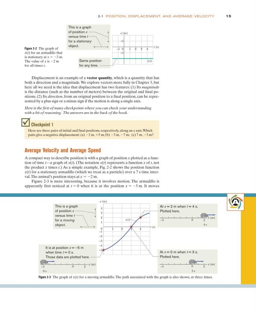
Figure 2-3 is more interesting, because it involves motion. The armadillo is
apparently first noticed at t ϭ 0 when it is at the position x ϭ Ϫ5 m. It moves
Figure 2-2 The graph of
x(t) for an armadillo that
is stationary at x ϭ Ϫ2 m.
The value of x is Ϫ2 m
for all times t.
x (m)
t (s)
1 2 3 4
+1
–1
–1
x(t)
0
This is a graph
of position x
versus time t
for a stationary
object.
Same position
for any time.
Figure 2-3 The graph of x(t) for a moving armadillo. The path associated with the graph is also shown, at three times.
x (m)
t (s)
1
2
3
4
4
3
2
1
0
It is at position x = –5 m
when time t = 0 s.
Those data are plotted here.
This is a graph
of position x
versus time t
for a moving
object.
0
–5
2
x (m)
0 s
0
–5
2
x (m)
3 s
At x = 0 m when t = 3 s.
Plotted here.
At x = 2 m when t = 4 s.
Plotted here.
–1
–2
–3
–4
–5
x(t)
0
–5
2
x (m)
4 s
A
both a direction and a magnitude. We explore vectors more fully in Chapter 3, but
here all we need is the idea that displacement has two features: (1) Its magnitude
is the distance (such as the number of meters) between the original and final positions. (2) Its direction, from an original position to a final position, can be represented by a plus sign or a minus sign if the motion is along a single axis.
Here is the first of many checkpoints where you can check your understanding
with a bit of reasoning. The answers are in the back of the book.
15
2-1 POSITION, DISPL ACE M E NT, AN D AVE RAG E VE LOCITY
Checkpoint 1
Here are three pairs of initial and final positions, respectively, along an x axis. Which
pairs give a negative displacement: (a) Ϫ3 m, ϩ5 m; (b) Ϫ3 m, Ϫ7 m; (c) 7 m, Ϫ3 m?
Average Velocity and Average Speed
A compact way to describe position is with a graph of position x plotted as a function of time t—a graph of x(t). (The notation x(t) represents a function x of t, not
the product x times t.) As a simple example, Fig. 2-2 shows the position function
x(t) for a stationary armadillo (which we treat as a particle) over a 7 s time interval. The animal’s position stays at x ϭ Ϫ2 m.
Figure 2-3 is more interesting, because it involves motion. The armadillo is
apparently first noticed at t ϭ 0 when it is at the position x ϭ Ϫ5 m. It moves
Figure 2-2 The graph of
x(t) for an armadillo that
is stationary at x ϭ Ϫ2 m.
The value of x is Ϫ2 m
for all times t.
x (m)
t (s)
1 2 3 4
+1
–1
–1
x(t)
0
This is a graph
of position x
versus time t
for a stationary
object.
Same position
for any time.
Figure 2-3 The graph of x(t) for a moving armadillo. The path associated with the graph is also shown, at three times.
x (m)
t (s)
1
2
3
4
4
3
2
1
0
It is at position x = –5 m
when time t = 0 s.
Those data are plotted here.
This is a graph
of position x
versus time t
for a moving
object.
0
–5
2
x (m)
0 s
0
–5
2
x (m)
3 s
At x = 0 m when t = 3 s.
Plotted here.
At x = 2 m when t = 4 s.
Plotted here.
–1
–2
–3
–4
–5
x(t)
0
–5
2
x (m)
4 s
A