

163
7-5 WOR K DON E BY A G E N E RAL VAR IAB LE FORCE
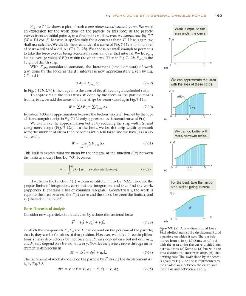
Figure 7-12 (a) A one-dimensional force
plotted against the displacement x of
a particle on which it acts. The particle
moves from x i to x f . (b) Same as (a) but
with the area under the curve divided into
narrow strips. (c) Same as (b) but with the
area divided into narrower strips. (d) The
limiting case. The work done by the force
is given by Eq. 7-32 and is represented by
the shaded area between the curve and
the x axis and between x i and x f .
F
:
(x)
Figure 7-12a shows a plot of such a one-dimensional variable force. We want
an expression for the work done on the particle by this force as the particle
moves from an initial point x i to a final point x f . However, we cannot use Eq. 7-7
(W ϭ Fd cos f) because it applies only for a constant force . Here, again, we
shall use calculus. We divide the area under the curve of Fig. 7-12a into a number
of narrow strips of width ⌬x (Fig. 7-12b). We choose ⌬x small enough to permit us
to take the force F(x) as being reasonably constant over that interval. We let F j,avg
be the average value of F(x) within the jth interval. Then in Fig. 7-12b, F j,avg is the
height of the jth strip.
With F j,avg considered constant, the increment (small amount) of work
⌬W j done by the force in the jth interval is now approximately given by Eq.
7-7 and is
⌬W j ϭ F j,avg ⌬x.
(7-29)
In Fig. 7-12b, ⌬W j is then equal to the area of the jth rectangular, shaded strip.
To approximate the total work W done by the force as the particle moves
from x i to x f , we add the areas of all the strips between x i and x f in Fig. 7-12b:
W ϭ
ϭ
⌬ x.
( 7 - 3 0 )
Equation 7-30 is an approximation because the broken “skyline” formed by the tops
of the rectangular strips in Fig. 7-12b only approximates the actual curve of F(x).
We can make the approximation better by reducing the strip width ⌬x and
using more strips (Fig. 7-12c). In the limit, we let the strip width approach
zero; the number of strips then becomes infinitely large and we have, as an exact result,
(7-31)
This limit is exactly what we mean by the integral of the function F(x) between
the limits x i and x f .Thus, Eq. 7-31 becomes
(work: variable force).
(7-32)
If we know the function F(x), we can substitute it into Eq. 7-32, introduce the
proper limits of integration, carry out the integration, and thus find the work.
(Appendix E contains a list of common integrals.) Geometrically, the work is
equal to the area between the F(x) curve and the x axis, between the limits x i and
x f (shaded in Fig. 7-12d).
Three-Dimensional Analysis
Consider now a particle that is acted on by a three-dimensional force
ϭ F x ϩ F y ϩ F z ,
( 7 - 3 3 )
in which the components F x , F y , and F z can depend on the position of the particle;
that is, they can be functions of that position. However, we make three simplifications: F x may depend on x but not on y or z, F y may depend on y but not on x or z,
and F z may depend on z but not on x or y. Now let the particle move through an incremental displacement
ϭ dx ϩ dy ϩ dz .
( 7 - 3 4 )
The increment of work dW done on the particle by during the displacement
is, by Eq. 7-8,
(7-35)
dW ϭ F
: ؒ dr
: ϭ F x dx ϩ F y dy ϩ F z dz.
dr
:
F
:
k ˆ
j
ˆ
i
ˆ
dr
:
k ˆ
j
ˆ
i
ˆ
F
:
W ϭ ͵
x f
x i
F(x) dx
W ϭ lim
⌬x : 0
͚ F j,avg ⌬ x.
͚ F j,avg
͚ ⌬W j
F
:
F(x)
x
x i
x f
0
(a)
Work is equal to the
area under the curve.
F(x)
x
x i
x f
F j, avg
∆ x
0
(b)
∆W j
We can approximate that area
with the area of these strips.
F(x)
x
x i
x f
0
∆ x
(c)
We can do better with
more, narrower strips.
F(x)
x
x i
x f
0
W
(d)
For the best, take the limit of
strip widths going to zero.
7-5 WOR K DON E BY A G E N E RAL VAR IAB LE FORCE
Figure 7-12 (a) A one-dimensional force
plotted against the displacement x of
a particle on which it acts. The particle
moves from x i to x f . (b) Same as (a) but
with the area under the curve divided into
narrow strips. (c) Same as (b) but with the
area divided into narrower strips. (d) The
limiting case. The work done by the force
is given by Eq. 7-32 and is represented by
the shaded area between the curve and
the x axis and between x i and x f .
F
:
(x)
Figure 7-12a shows a plot of such a one-dimensional variable force. We want
an expression for the work done on the particle by this force as the particle
moves from an initial point x i to a final point x f . However, we cannot use Eq. 7-7
(W ϭ Fd cos f) because it applies only for a constant force . Here, again, we
shall use calculus. We divide the area under the curve of Fig. 7-12a into a number
of narrow strips of width ⌬x (Fig. 7-12b). We choose ⌬x small enough to permit us
to take the force F(x) as being reasonably constant over that interval. We let F j,avg
be the average value of F(x) within the jth interval. Then in Fig. 7-12b, F j,avg is the
height of the jth strip.
With F j,avg considered constant, the increment (small amount) of work
⌬W j done by the force in the jth interval is now approximately given by Eq.
7-7 and is
⌬W j ϭ F j,avg ⌬x.
(7-29)
In Fig. 7-12b, ⌬W j is then equal to the area of the jth rectangular, shaded strip.
To approximate the total work W done by the force as the particle moves
from x i to x f , we add the areas of all the strips between x i and x f in Fig. 7-12b:
W ϭ
ϭ
⌬ x.
( 7 - 3 0 )
Equation 7-30 is an approximation because the broken “skyline” formed by the tops
of the rectangular strips in Fig. 7-12b only approximates the actual curve of F(x).
We can make the approximation better by reducing the strip width ⌬x and
using more strips (Fig. 7-12c). In the limit, we let the strip width approach
zero; the number of strips then becomes infinitely large and we have, as an exact result,
(7-31)
This limit is exactly what we mean by the integral of the function F(x) between
the limits x i and x f .Thus, Eq. 7-31 becomes
(work: variable force).
(7-32)
If we know the function F(x), we can substitute it into Eq. 7-32, introduce the
proper limits of integration, carry out the integration, and thus find the work.
(Appendix E contains a list of common integrals.) Geometrically, the work is
equal to the area between the F(x) curve and the x axis, between the limits x i and
x f (shaded in Fig. 7-12d).
Three-Dimensional Analysis
Consider now a particle that is acted on by a three-dimensional force
ϭ F x ϩ F y ϩ F z ,
( 7 - 3 3 )
in which the components F x , F y , and F z can depend on the position of the particle;
that is, they can be functions of that position. However, we make three simplifications: F x may depend on x but not on y or z, F y may depend on y but not on x or z,
and F z may depend on z but not on x or y. Now let the particle move through an incremental displacement
ϭ dx ϩ dy ϩ dz .
( 7 - 3 4 )
The increment of work dW done on the particle by during the displacement
is, by Eq. 7-8,
(7-35)
dW ϭ F
: ؒ dr
: ϭ F x dx ϩ F y dy ϩ F z dz.
dr
:
F
:
k ˆ
j
ˆ
i
ˆ
dr
:
k ˆ
j
ˆ
i
ˆ
F
:
W ϭ ͵
x f
x i
F(x) dx
W ϭ lim
⌬x : 0
͚ F j,avg ⌬ x.
͚ F j,avg
͚ ⌬W j
F
:
F(x)
x
x i
x f
0
(a)
Work is equal to the
area under the curve.
F(x)
x
x i
x f
F j, avg
∆ x
0
(b)
∆W j
We can approximate that area
with the area of these strips.
F(x)
x
x i
x f
0
∆ x
(c)
We can do better with
more, narrower strips.
F(x)
x
x i
x f
0
W
(d)
For the best, take the limit of
strip widths going to zero.