

3.3 Branching (if, elif and else)
7 3
d = 1
# step length (e.g., in meter)
x = np.zeros(N+1)
# x coordinates
y = np.zeros(N+1)
# y coordinates
x[0] = 0; y[0] = 0
# set initial position
for i in range(0, N, 1):
r = random.random()
# random number in [0,1)
if 0 <= r < 0.25:
# move north
y[i+1] = y[i] + d
x[i+1] = x[i]
elif 0.25 <= r < 0.5:
# move east
x[i+1] = x[i] + d
y[i+1] = y[i]
elif 0.5 <= r < 0.75:
# move south
y[i+1] = y[i] - d
x[i+1] = x[i]
else:
# move west
x[i+1] = x[i] - d
y[i+1] = y[i]
# plot path (mark start and stop with blue o and *, respectively)
plt.plot(x, y, ’r--’, x[0], y[0], ’bo’, x[-1], y[-1], ’b*’)
plt.xlabel(’x’); plt.ylabel(’y’)
plt.show()
Here, the initial position is explicitly set, even if x[0] and y[0] are known to
be zero already. We do this, since the initial position is important, and by setting it
explicitly, it is clearly not accidental what the starting position is. Note that if a step
is taken in the x-direction, the y-coordinate is unchanged, and vice versa.
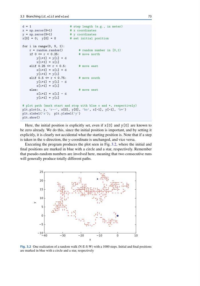
Executing the program produces the plot seen in Fig. 3.2, where the initial and
final positions are marked in blue with a circle and a star, respectively. Remember
that pseudo-random numbers are involved here, meaning that two consecutive runs
will generally produce totally different paths.
Fig. 3.2 One realization of a random walk (N-E-S-W) with a 1000 steps. Initial and final positions
are marked in blue with a circle and a star, respectively
7 3
d = 1
# step length (e.g., in meter)
x = np.zeros(N+1)
# x coordinates
y = np.zeros(N+1)
# y coordinates
x[0] = 0; y[0] = 0
# set initial position
for i in range(0, N, 1):
r = random.random()
# random number in [0,1)
if 0 <= r < 0.25:
# move north
y[i+1] = y[i] + d
x[i+1] = x[i]
elif 0.25 <= r < 0.5:
# move east
x[i+1] = x[i] + d
y[i+1] = y[i]
elif 0.5 <= r < 0.75:
# move south
y[i+1] = y[i] - d
x[i+1] = x[i]
else:
# move west
x[i+1] = x[i] - d
y[i+1] = y[i]
# plot path (mark start and stop with blue o and *, respectively)
plt.plot(x, y, ’r--’, x[0], y[0], ’bo’, x[-1], y[-1], ’b*’)
plt.xlabel(’x’); plt.ylabel(’y’)
plt.show()
Here, the initial position is explicitly set, even if x[0] and y[0] are known to
be zero already. We do this, since the initial position is important, and by setting it
explicitly, it is clearly not accidental what the starting position is. Note that if a step
is taken in the x-direction, the y-coordinate is unchanged, and vice versa.
Executing the program produces the plot seen in Fig. 3.2, where the initial and
final positions are marked in blue with a circle and a star, respectively. Remember
that pseudo-random numbers are involved here, meaning that two consecutive runs
will generally produce totally different paths.
Fig. 3.2 One realization of a random walk (N-E-S-W) with a 1000 steps. Initial and final positions
are marked in blue with a circle and a star, respectively