

9.3 Exercises
305
3. The backward 2-step method with Δt = 0.01
Choose the model problem from Sect. 9.2.4.
Filename: rod_BE_vs_B2Step.py.
Exercise 9.4: Explore Adaptive and Implicit Methods
We consider the same problem as in Exercise 9.2. Now we want to explore the use of
adaptive and implicit methods from Odespy to see if they are more efficient than the
Forward Euler method. Assume that you want the accuracy provided by the Forward
Euler method with its maximum Δt value. Since there exists an analytical solution,
you can compute an error measure that summarizes the error in space and time over
the whole simulation:
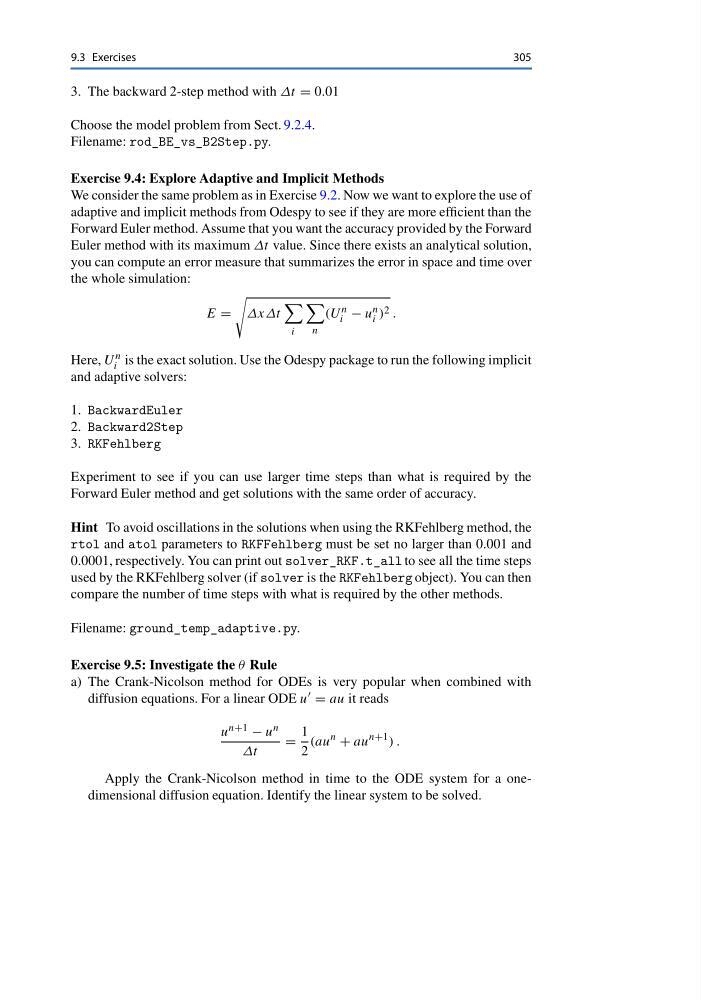
E =
ΔxΔt
i
n
(U n
i − u n
i ) 2 .
Here, U
n
i is the exact solution. Use the Odespy package to run the following implicit
and adaptive solvers:
1. BackwardEuler
2. Backward2Step
3. RKFehlberg
Experiment to see if you can use larger time steps than what is required by the
Forward Euler method and get solutions with the same order of accuracy.
Hint To avoid oscillations in the solutions when using the RKFehlberg method, the
rtol and atol parameters to RKFFehlberg must be set no larger than 0.001 and
0.0001, respectively. You can print out solver_RKF.t_all to see all the time steps
used by the RKFehlberg solver (if solver is the RKFehlberg object). You can then
compare the number of time steps with what is required by the other methods.
Filename: ground_temp_adaptive.py.
Exercise 9.5: Investigate the θ Rule
a) The Crank-Nicolson method for ODEs is very popular when combined with
diffusion equations. For a linear ODE u = au it reads
u n+1 − u n
Δt
=
1
2
(au
n
+ au
n+1 ) .
Apply the Crank-Nicolson method in time to the ODE system for a onedimensional diffusion equation. Identify the linear system to be solved.
305
3. The backward 2-step method with Δt = 0.01
Choose the model problem from Sect. 9.2.4.
Filename: rod_BE_vs_B2Step.py.
Exercise 9.4: Explore Adaptive and Implicit Methods
We consider the same problem as in Exercise 9.2. Now we want to explore the use of
adaptive and implicit methods from Odespy to see if they are more efficient than the
Forward Euler method. Assume that you want the accuracy provided by the Forward
Euler method with its maximum Δt value. Since there exists an analytical solution,
you can compute an error measure that summarizes the error in space and time over
the whole simulation:
E =
ΔxΔt
i
n
(U n
i − u n
i ) 2 .
Here, U
n
i is the exact solution. Use the Odespy package to run the following implicit
and adaptive solvers:
1. BackwardEuler
2. Backward2Step
3. RKFehlberg
Experiment to see if you can use larger time steps than what is required by the
Forward Euler method and get solutions with the same order of accuracy.
Hint To avoid oscillations in the solutions when using the RKFehlberg method, the
rtol and atol parameters to RKFFehlberg must be set no larger than 0.001 and
0.0001, respectively. You can print out solver_RKF.t_all to see all the time steps
used by the RKFehlberg solver (if solver is the RKFehlberg object). You can then
compare the number of time steps with what is required by the other methods.
Filename: ground_temp_adaptive.py.
Exercise 9.5: Investigate the θ Rule
a) The Crank-Nicolson method for ODEs is very popular when combined with
diffusion equations. For a linear ODE u = au it reads
u n+1 − u n
Δt
=
1
2
(au
n
+ au
n+1 ) .
Apply the Crank-Nicolson method in time to the ODE system for a onedimensional diffusion equation. Identify the linear system to be solved.