

262
8 Solving Ordinary Differential Equations
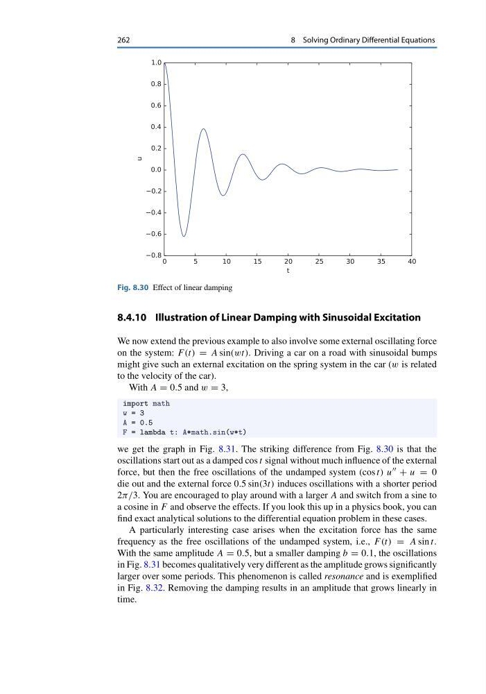
Fig. 8.30 Effect of linear damping
8.4.10 Illustration of Linear Damping with Sinusoidal Excitation
We now extend the previous example to also involve some external oscillating force
on the system: F (t) = A sin(wt). Driving a car on a road with sinusoidal bumps
might give such an external excitation on the spring system in the car (w is related
to the velocity of the car).
With A = 0.5 and w = 3,
import math
w = 3
A = 0.5
F = lambda t: A*math.sin(w*t)
we get the graph in Fig. 8.31. The striking difference from Fig. 8.30 is that the
oscillations start out as a damped cos t signal without much influence of the external
force, but then the free oscillations of the undamped system (cos t) u + u = 0
die out and the external force 0.5 sin(3t) induces oscillations with a shorter period
2π/3. You are encouraged to play around with a larger A and switch from a sine to
a cosine in F and observe the effects. If you look this up in a physics book, you can
find exact analytical solutions to the differential equation problem in these cases.
A particularly interesting case arises when the excitation force has the same
frequency as the free oscillations of the undamped system, i.e., F (t) = A sin t.
With the same amplitude A = 0.5, but a smaller damping b = 0.1, the oscillations
in Fig. 8.31 becomes qualitatively very different as the amplitude grows significantly
larger over some periods. This phenomenon is called resonance and is exemplified
in Fig. 8.32. Removing the damping results in an amplitude that grows linearly in
time.
8 Solving Ordinary Differential Equations
Fig. 8.30 Effect of linear damping
8.4.10 Illustration of Linear Damping with Sinusoidal Excitation
We now extend the previous example to also involve some external oscillating force
on the system: F (t) = A sin(wt). Driving a car on a road with sinusoidal bumps
might give such an external excitation on the spring system in the car (w is related
to the velocity of the car).
With A = 0.5 and w = 3,
import math
w = 3
A = 0.5
F = lambda t: A*math.sin(w*t)
we get the graph in Fig. 8.31. The striking difference from Fig. 8.30 is that the
oscillations start out as a damped cos t signal without much influence of the external
force, but then the free oscillations of the undamped system (cos t) u + u = 0
die out and the external force 0.5 sin(3t) induces oscillations with a shorter period
2π/3. You are encouraged to play around with a larger A and switch from a sine to
a cosine in F and observe the effects. If you look this up in a physics book, you can
find exact analytical solutions to the differential equation problem in these cases.
A particularly interesting case arises when the excitation force has the same
frequency as the free oscillations of the undamped system, i.e., F (t) = A sin t.
With the same amplitude A = 0.5, but a smaller damping b = 0.1, the oscillations
in Fig. 8.31 becomes qualitatively very different as the amplitude grows significantly
larger over some periods. This phenomenon is called resonance and is exemplified
in Fig. 8.32. Removing the damping results in an amplitude that grows linearly in
time.