

250
8 Solving Ordinary Differential Equations
Odespy: Example with Oscillations Using Odespy to solve oscillation ODEs like
u + ω 2 u = 0, reformulated as a system u = v and v = −ω 2 u, can be done with
the following code:
import odespy
import numpy as np
import matplotlib.pyplot as plt
# Define the ODE system
# u’ = v
# v’ = -omega**2*u
def f(sol, t, omega=2):
u, v = sol
return [v, -omega**2*u]
# Set and compute problem dependent parameters
omega = 2
X_0 = 1
number_of_periods = 40
time_steps_per_period = 20
P = 2*np.pi/omega
# length of one period
dt = P/time_steps_per_period
# time step
T = number_of_periods*P
# final simulation time
# Create Odespy solver object
odespy_method = odespy.RK2
solver = odespy_method(f, f_args=[omega])
# The initial condition for the system is collected in a list
solver.set_initial_condition([X_0, 0])
# Compute the desired time points where we want the solution
N_t = int(round(T/dt))
# no of time intervals
time_points = np.linspace(0, T, N_t+1)
# Solve the ODE problem
sol, t = solver.solve(time_points)
# Note: sol contains both displacement and velocity
# Extract original variables
u = sol[:,0]
v = sol[:,1]
plt.plot(t, u, t, v) # ...for a quick check on u and v
plt.show()
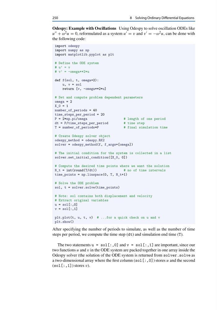
After specifying the number of periods to simulate, as well as the number of time
steps per period, we compute the time step (dt) and simulation end time (T).
The two statements u = sol[:,0] and v = sol[:,1] are important, since our
two functions u and v in the ODE system are packed together in one array inside the
Odespy solver (the solution of the ODE system is returned from solver.solve as
a two-dimensional array where the first column (sol[:,0]) stores u and the second
(sol[:,1]) stores v).
8 Solving Ordinary Differential Equations
Odespy: Example with Oscillations Using Odespy to solve oscillation ODEs like
u + ω 2 u = 0, reformulated as a system u = v and v = −ω 2 u, can be done with
the following code:
import odespy
import numpy as np
import matplotlib.pyplot as plt
# Define the ODE system
# u’ = v
# v’ = -omega**2*u
def f(sol, t, omega=2):
u, v = sol
return [v, -omega**2*u]
# Set and compute problem dependent parameters
omega = 2
X_0 = 1
number_of_periods = 40
time_steps_per_period = 20
P = 2*np.pi/omega
# length of one period
dt = P/time_steps_per_period
# time step
T = number_of_periods*P
# final simulation time
# Create Odespy solver object
odespy_method = odespy.RK2
solver = odespy_method(f, f_args=[omega])
# The initial condition for the system is collected in a list
solver.set_initial_condition([X_0, 0])
# Compute the desired time points where we want the solution
N_t = int(round(T/dt))
# no of time intervals
time_points = np.linspace(0, T, N_t+1)
# Solve the ODE problem
sol, t = solver.solve(time_points)
# Note: sol contains both displacement and velocity
# Extract original variables
u = sol[:,0]
v = sol[:,1]
plt.plot(t, u, t, v) # ...for a quick check on u and v
plt.show()
After specifying the number of periods to simulate, as well as the number of time
steps per period, we compute the time step (dt) and simulation end time (T).
The two statements u = sol[:,0] and v = sol[:,1] are important, since our
two functions u and v in the ODE system are packed together in one array inside the
Odespy solver (the solution of the ODE system is returned from solver.solve as
a two-dimensional array where the first column (sol[:,0]) stores u and the second
(sol[:,1]) stores v).