

240
8 Solving Ordinary Differential Equations
where ω is a given physical parameter. Equation (8.40) models a one-dimensional
system oscillating without damping (i.e., with negligible damping). Onedimensional here means that some motion takes place along one dimension only in
some coordinate system. Along with (8.40) we need the two initial conditions u(0)
and u (0).
8.4.1 Derivation of a Simple Model
Many engineering systems undergo oscillations, and differential equations constitute the key tool to understand, predict, and control the oscillations. We start with
the simplest possible model that captures the essential dynamics of an oscillating
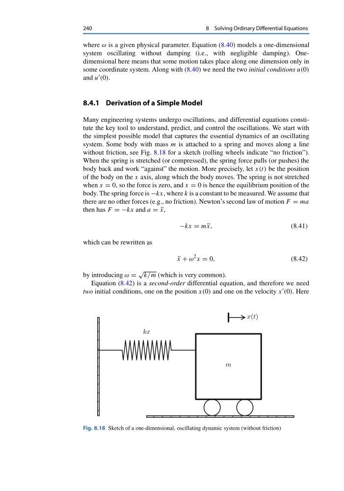
system. Some body with mass m is attached to a spring and moves along a line
without friction, see Fig. 8.18 for a sketch (rolling wheels indicate “no friction”).
When the spring is stretched (or compressed), the spring force pulls (or pushes) the
body back and work “against” the motion. More precisely, let x(t) be the position
of the body on the x axis, along which the body moves. The spring is not stretched
when x = 0, so the force is zero, and x = 0 is hence the equilibrium position of the
body. The spring force is −kx, where k is a constant to be measured. We assume that
there are no other forces (e.g., no friction). Newton’s second law of motion F = ma
then has F = −kx and a = ¨
x,
−kx = m ¨
x,
(8.41)
which can be rewritten as
¨
x + ω
2 x = 0,
(8.42)
by introducing ω =
√
k/m (which is very common).
Equation (8.42) is a second-order differential equation, and therefore we need
two initial conditions, one on the position x(0) and one on the velocity x (0). Here
Fig. 8.18 Sketch of a one-dimensional, oscillating dynamic system (without friction)
8 Solving Ordinary Differential Equations
where ω is a given physical parameter. Equation (8.40) models a one-dimensional
system oscillating without damping (i.e., with negligible damping). Onedimensional here means that some motion takes place along one dimension only in
some coordinate system. Along with (8.40) we need the two initial conditions u(0)
and u (0).
8.4.1 Derivation of a Simple Model
Many engineering systems undergo oscillations, and differential equations constitute the key tool to understand, predict, and control the oscillations. We start with
the simplest possible model that captures the essential dynamics of an oscillating
system. Some body with mass m is attached to a spring and moves along a line
without friction, see Fig. 8.18 for a sketch (rolling wheels indicate “no friction”).
When the spring is stretched (or compressed), the spring force pulls (or pushes) the
body back and work “against” the motion. More precisely, let x(t) be the position
of the body on the x axis, along which the body moves. The spring is not stretched
when x = 0, so the force is zero, and x = 0 is hence the equilibrium position of the
body. The spring force is −kx, where k is a constant to be measured. We assume that
there are no other forces (e.g., no friction). Newton’s second law of motion F = ma
then has F = −kx and a = ¨
x,
−kx = m ¨
x,
(8.41)
which can be rewritten as
¨
x + ω
2 x = 0,
(8.42)
by introducing ω =
√
k/m (which is very common).
Equation (8.42) is a second-order differential equation, and therefore we need
two initial conditions, one on the position x(0) and one on the velocity x (0). Here
Fig. 8.18 Sketch of a one-dimensional, oscillating dynamic system (without friction)