

234
8 Solving Ordinary Differential Equations
The list version looks a bit nicer, so that is why we prefer a list and rather introduce
f_ = lambda u, t: asarray(f(u,t)) in the general ode_FE function.
We can now show a function that runs the previous SIR example, while using the
generic ode_FE function:
def demo_SIR():
"""Test case using a SIR model."""
def f(u, t):
S, I, R = u
return [-beta*S*I, beta*S*I - gamma*I, gamma*I]
beta = 10./(40*8*24)
gamma = 3./(15*24)
dt = 0.1
# 6 min
D = 30
# Simulate for D days
N_t = int(D*24/dt)
# Corresponding no of time steps
T = dt*N_t
# End time
U_0 = [50, 1, 0]
u, t = ode_FE(f, U_0, dt, T)
S = u[:,0]
I = u[:,1]
R = u[:,2]
fig = plt.figure()
l1, l2, l3 = plt.plot(t, S, t, I, t, R)
fig.legend((l1, l2, l3), (’S’, ’I’, ’R’), ’center right’)
plt.xlabel(’hours’)
plt.show()
# Consistency check:
N = S[0] + I[0] + R[0]
eps = 1E-12 # Tolerance for comparing real numbers
for n in range(len(S)):
SIR_sum = S[n] + I[n] + R[n]
if abs(SIR_sum - N) > eps:
print(’*** consistency check failed: S+I+R={:g} != {:g}’\
.format(SIR_sum, N))
if __name__ == ’__main__’:
demo_SIR()
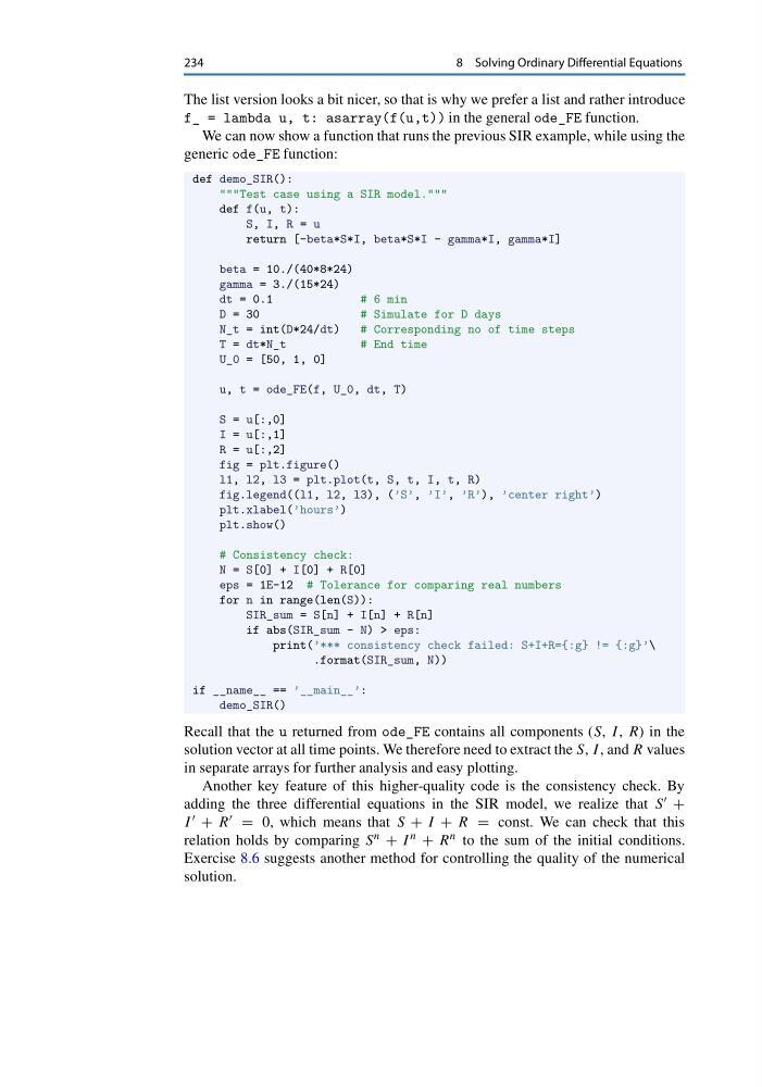
Recall that the u returned from ode_FE contains all components (S, I , R) in the
solution vector at all time points. We therefore need to extract the S, I , and R values
in separate arrays for further analysis and easy plotting.
Another key feature of this higher-quality code is the consistency check. By
adding the three differential equations in the SIR model, we realize that S +
I + R = 0, which means that S + I + R = const. We can check that this
relation holds by comparing S n + I n + R n to the sum of the initial conditions.
Exercise 8.6 suggests another method for controlling the quality of the numerical
solution.
8 Solving Ordinary Differential Equations
The list version looks a bit nicer, so that is why we prefer a list and rather introduce
f_ = lambda u, t: asarray(f(u,t)) in the general ode_FE function.
We can now show a function that runs the previous SIR example, while using the
generic ode_FE function:
def demo_SIR():
"""Test case using a SIR model."""
def f(u, t):
S, I, R = u
return [-beta*S*I, beta*S*I - gamma*I, gamma*I]
beta = 10./(40*8*24)
gamma = 3./(15*24)
dt = 0.1
# 6 min
D = 30
# Simulate for D days
N_t = int(D*24/dt)
# Corresponding no of time steps
T = dt*N_t
# End time
U_0 = [50, 1, 0]
u, t = ode_FE(f, U_0, dt, T)
S = u[:,0]
I = u[:,1]
R = u[:,2]
fig = plt.figure()
l1, l2, l3 = plt.plot(t, S, t, I, t, R)
fig.legend((l1, l2, l3), (’S’, ’I’, ’R’), ’center right’)
plt.xlabel(’hours’)
plt.show()
# Consistency check:
N = S[0] + I[0] + R[0]
eps = 1E-12 # Tolerance for comparing real numbers
for n in range(len(S)):
SIR_sum = S[n] + I[n] + R[n]
if abs(SIR_sum - N) > eps:
print(’*** consistency check failed: S+I+R={:g} != {:g}’\
.format(SIR_sum, N))
if __name__ == ’__main__’:
demo_SIR()
Recall that the u returned from ode_FE contains all components (S, I , R) in the
solution vector at all time points. We therefore need to extract the S, I , and R values
in separate arrays for further analysis and easy plotting.
Another key feature of this higher-quality code is the consistency check. By
adding the three differential equations in the SIR model, we realize that S +
I + R = 0, which means that S + I + R = const. We can check that this
relation holds by comparing S n + I n + R n to the sum of the initial conditions.
Exercise 8.6 suggests another method for controlling the quality of the numerical
solution.