

8.3 Spreading of Disease: A System of First Order ODEs
227
and I categories. The probability that people meet in pairs during a time T is (by
the empirical frequency definition of probability) equal to m/n, i.e., the number
of successes divided by the number of possible outcomes. From such statistics we
normally derive quantities expressed per unit time, i.e., here we want the probability
per unit time, μ, which is found from dividing by T : μ = m/(nT ).
Given the probability μ, the expected number of meetings per time interval of
SI possible pairs of people is (from basic statistics) μSI . During a time interval
Δt, there will be μSI Δt expected number of meetings between susceptibles and
infected people such that the virus may spread. Only a fraction of the μΔtSI
meetings are effective in the sense that the susceptible actually becomes infected.
Counting that m people get infected in n such pairwise meetings (say 5 are infected
from 1000 meetings), we can estimate the probability of being infected as p = m/n.
The expected number of individuals in the S category that in a time interval Δt catch
the virus and get infected is then pμΔtSI . Introducing a new constant β = pμ to
save some writing, we arrive at the formula βΔtSI .
The value of β must be known in order to predict the future with the disease
model. One possibility is to estimate p and μ from their meanings in the derivation
above. Alternatively, we can observe an “experiment” where there are S 0 susceptibles and I 0 infected at some point in time. During a time interval T we count that N
susceptibles have become infected. Using (8.9) as a rough approximation of how S
has developed during time T (and now T is not necessarily small, but we use (8.9)
anyway), we get
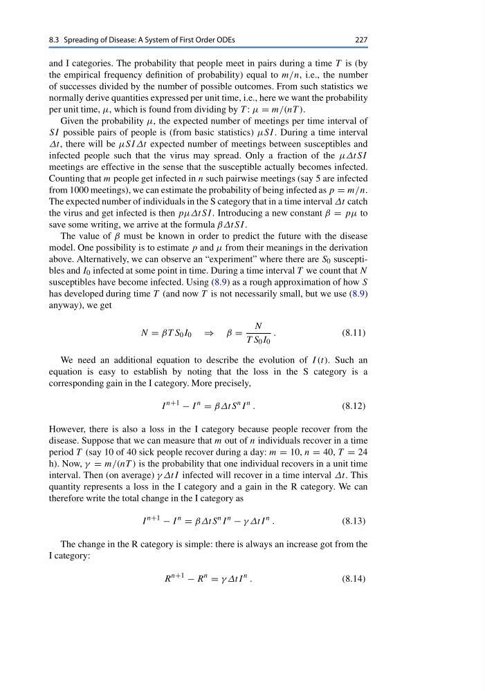
N = βT S 0 I 0 ⇒ β =
N
T S 0 I 0
.
(8.11)
We need an additional equation to describe the evolution of I (t). Such an
equation is easy to establish by noting that the loss in the S category is a
corresponding gain in the I category. More precisely,
I
n+1
− I
n
= βΔtS
n I
n .
(8.12)
However, there is also a loss in the I category because people recover from the
disease. Suppose that we can measure that m out of n individuals recover in a time
period T (say 10 of 40 sick people recover during a day: m = 10, n = 40, T = 24
h). Now, γ = m/(nT ) is the probability that one individual recovers in a unit time
interval. Then (on average) γ ΔtI infected will recover in a time interval Δt. This
quantity represents a loss in the I category and a gain in the R category. We can
therefore write the total change in the I category as
I
n+1
− I
n
= βΔtS
n I
n
− γ ΔtI
n .
(8.13)
The change in the R category is simple: there is always an increase got from the
I category:
R
n+1
− R
n
= γ ΔtI
n .
(8.14)
227
and I categories. The probability that people meet in pairs during a time T is (by
the empirical frequency definition of probability) equal to m/n, i.e., the number
of successes divided by the number of possible outcomes. From such statistics we
normally derive quantities expressed per unit time, i.e., here we want the probability
per unit time, μ, which is found from dividing by T : μ = m/(nT ).
Given the probability μ, the expected number of meetings per time interval of
SI possible pairs of people is (from basic statistics) μSI . During a time interval
Δt, there will be μSI Δt expected number of meetings between susceptibles and
infected people such that the virus may spread. Only a fraction of the μΔtSI
meetings are effective in the sense that the susceptible actually becomes infected.
Counting that m people get infected in n such pairwise meetings (say 5 are infected
from 1000 meetings), we can estimate the probability of being infected as p = m/n.
The expected number of individuals in the S category that in a time interval Δt catch
the virus and get infected is then pμΔtSI . Introducing a new constant β = pμ to
save some writing, we arrive at the formula βΔtSI .
The value of β must be known in order to predict the future with the disease
model. One possibility is to estimate p and μ from their meanings in the derivation
above. Alternatively, we can observe an “experiment” where there are S 0 susceptibles and I 0 infected at some point in time. During a time interval T we count that N
susceptibles have become infected. Using (8.9) as a rough approximation of how S
has developed during time T (and now T is not necessarily small, but we use (8.9)
anyway), we get
N = βT S 0 I 0 ⇒ β =
N
T S 0 I 0
.
(8.11)
We need an additional equation to describe the evolution of I (t). Such an
equation is easy to establish by noting that the loss in the S category is a
corresponding gain in the I category. More precisely,
I
n+1
− I
n
= βΔtS
n I
n .
(8.12)
However, there is also a loss in the I category because people recover from the
disease. Suppose that we can measure that m out of n individuals recover in a time
period T (say 10 of 40 sick people recover during a day: m = 10, n = 40, T = 24
h). Now, γ = m/(nT ) is the probability that one individual recovers in a unit time
interval. Then (on average) γ ΔtI infected will recover in a time interval Δt. This
quantity represents a loss in the I category and a gain in the R category. We can
therefore write the total change in the I category as
I
n+1
− I
n
= βΔtS
n I
n
− γ ΔtI
n .
(8.13)
The change in the R category is simple: there is always an increase got from the
I category:
R
n+1
− R
n
= γ ΔtI
n .
(8.14)