

8.2 Population Growth: A First Order ODE
211
easily deal with almost any differential equation! This is exactly the topic of the
present chapter.
8.2.1 Derivation of the Model
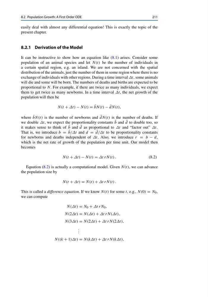
It can be instructive to show how an equation like (8.1) arises. Consider some
population of an animal species and let N(t) be the number of individuals in
a certain spatial region, e.g. an island. We are not concerned with the spatial
distribution of the animals, just the number of them in some region where there is no
exchange of individuals with other regions. During a time interval Δt, some animals
will die and some will be born. The numbers of deaths and births are expected to be
proportional to N. For example, if there are twice as many individuals, we expect
them to get twice as many newborns. In a time interval Δt, the net growth of the
population will then be
N(t + Δt) − N(t) = ¯
bN(t) − ¯
dN(t),
where ¯
bN(t) is the number of newborns and ¯
dN(t) is the number of deaths. If
we double Δt, we expect the proportionality constants ¯
b and ¯
d to double too, so
it makes sense to think of ¯
b and ¯
d as proportional to Δt and “factor out” Δt.
That is, we introduce b = ¯
b/Δt and d = ¯
d/Δt to be proportionality constants
for newborns and deaths independent of Δt. Also, we introduce r = b − d,
which is the net rate of growth of the population per time unit. Our model then
becomes
N(t + Δt) − N(t) = Δt rN(t) .
(8.2)
Equation (8.2) is actually a computational model. Given N(t), we can advance
the population size by
N(t + Δt) = N(t) + Δt rN(t) .
This is called a difference equation. If we know N(t) for some t, e.g., N(0) = N 0 ,
we can compute
N(Δt) = N 0 + Δt rN 0 ,
N(2Δt) = N(Δt) + Δt rN(Δt),
N(3Δt) = N(2Δt) + Δt rN(2Δt),
. . .
N((k + 1)Δt) = N(kΔt) + Δt rN(kΔt),
211
easily deal with almost any differential equation! This is exactly the topic of the
present chapter.
8.2.1 Derivation of the Model
It can be instructive to show how an equation like (8.1) arises. Consider some
population of an animal species and let N(t) be the number of individuals in
a certain spatial region, e.g. an island. We are not concerned with the spatial
distribution of the animals, just the number of them in some region where there is no
exchange of individuals with other regions. During a time interval Δt, some animals
will die and some will be born. The numbers of deaths and births are expected to be
proportional to N. For example, if there are twice as many individuals, we expect
them to get twice as many newborns. In a time interval Δt, the net growth of the
population will then be
N(t + Δt) − N(t) = ¯
bN(t) − ¯
dN(t),
where ¯
bN(t) is the number of newborns and ¯
dN(t) is the number of deaths. If
we double Δt, we expect the proportionality constants ¯
b and ¯
d to double too, so
it makes sense to think of ¯
b and ¯
d as proportional to Δt and “factor out” Δt.
That is, we introduce b = ¯
b/Δt and d = ¯
d/Δt to be proportionality constants
for newborns and deaths independent of Δt. Also, we introduce r = b − d,
which is the net rate of growth of the population per time unit. Our model then
becomes
N(t + Δt) − N(t) = Δt rN(t) .
(8.2)
Equation (8.2) is actually a computational model. Given N(t), we can advance
the population size by
N(t + Δt) = N(t) + Δt rN(t) .
This is called a difference equation. If we know N(t) for some t, e.g., N(0) = N 0 ,
we can compute
N(Δt) = N 0 + Δt rN 0 ,
N(2Δt) = N(Δt) + Δt rN(Δt),
N(3Δt) = N(2Δt) + Δt rN(2Δt),
. . .
N((k + 1)Δt) = N(kΔt) + Δt rN(kΔt),