

8.1 Filling a Water Tank: Two Cases
209
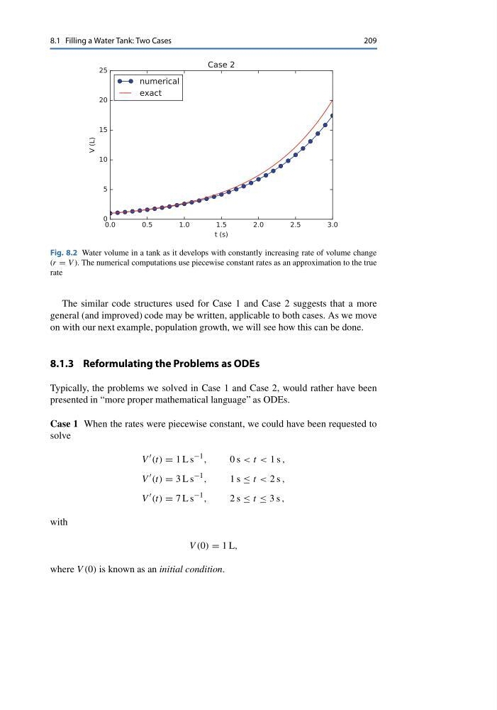
Fig. 8.2 Water volume in a tank as it develops with constantly increasing rate of volume change
(r = V ). The numerical computations use piecewise constant rates as an approximation to the true
rate
The similar code structures used for Case 1 and Case 2 suggests that a more
general (and improved) code may be written, applicable to both cases. As we move
on with our next example, population growth, we will see how this can be done.
8.1.3 Reformulating the Problems as ODEs
Typically, the problems we solved in Case 1 and Case 2, would rather have been
presented in “more proper mathematical language” as ODEs.
Case 1 When the rates were piecewise constant, we could have been requested to
solve
V
(t) = 1 L s
−1 ,
0 s < t < 1 s ,
V
(t) = 3 L s
−1 ,
1 s ≤ t < 2 s ,
V
(t) = 7 L s
−1 ,
2 s ≤ t ≤ 3 s ,
with
V (0) = 1 L,
where V (0) is known as an initial condition.
209
Fig. 8.2 Water volume in a tank as it develops with constantly increasing rate of volume change
(r = V ). The numerical computations use piecewise constant rates as an approximation to the true
rate
The similar code structures used for Case 1 and Case 2 suggests that a more
general (and improved) code may be written, applicable to both cases. As we move
on with our next example, population growth, we will see how this can be done.
8.1.3 Reformulating the Problems as ODEs
Typically, the problems we solved in Case 1 and Case 2, would rather have been
presented in “more proper mathematical language” as ODEs.
Case 1 When the rates were piecewise constant, we could have been requested to
solve
V
(t) = 1 L s
−1 ,
0 s < t < 1 s ,
V
(t) = 3 L s
−1 ,
1 s ≤ t < 2 s ,
V
(t) = 7 L s
−1 ,
2 s ≤ t ≤ 3 s ,
with
V (0) = 1 L,
where V (0) is known as an initial condition.