

206
8 Solving Ordinary Differential Equations
in the straight lines in between these points. Therefore, the exact solution is ready
and we may proceed to bring our reasoning into code.
Implementation and Performance A simple implementation may read
(rate_piecewise_constant.py):
import numpy as np
import matplotlib.pyplot as plt
a = 0.0; b = 3.0
# time interval
N = 3
# number of time steps
dt = (b - a)/N
# time step (s)
V_exact = [1.0, 2.0, 5.0, 12.0]
# exact volumes (L)
V = np.zeros(4)
# numerically computed volume (L)
V[0] = 1
# initial volume
r = np.zeros(3)
# rates of volume increase (L/s)
r[0] = 1; r[1] = 3; r[2] = 7
for i in [0, 1, 2]:
V[i+1] = V[i] + dt*r[i]
time = [0, 1, 2, 3]
plt.plot(time, V, ’bo-’, time, V_exact, ’r’)
plt.title(’Case 1’)
plt.legend([’numerical’,’exact’], loc=’upper left’)
plt.xlabel(’t (s)’)
plt.ylabel(’V (L)’)
plt.show()
As you can see, we have included the exact (hand computed) solution in the code,
so that it gets plotted together with the numerical solution found by the program.
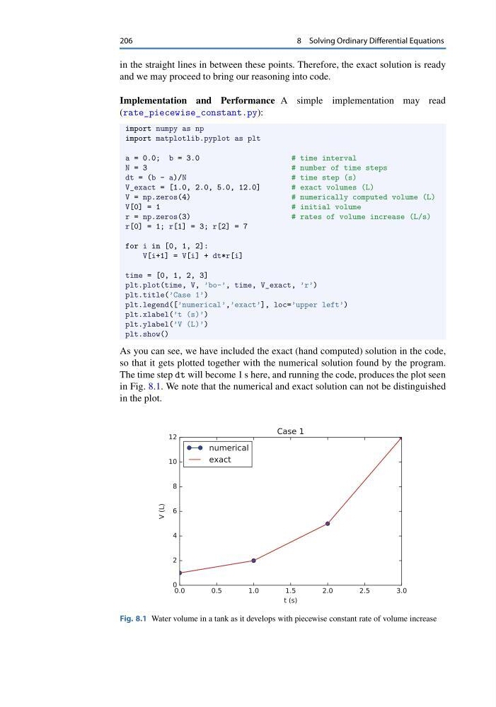
The time step dt will become 1 s here, and running the code, produces the plot seen
in Fig. 8.1. We note that the numerical and exact solution can not be distinguished
in the plot.
Fig. 8.1 Water volume in a tank as it develops with piecewise constant rate of volume increase
8 Solving Ordinary Differential Equations
in the straight lines in between these points. Therefore, the exact solution is ready
and we may proceed to bring our reasoning into code.
Implementation and Performance A simple implementation may read
(rate_piecewise_constant.py):
import numpy as np
import matplotlib.pyplot as plt
a = 0.0; b = 3.0
# time interval
N = 3
# number of time steps
dt = (b - a)/N
# time step (s)
V_exact = [1.0, 2.0, 5.0, 12.0]
# exact volumes (L)
V = np.zeros(4)
# numerically computed volume (L)
V[0] = 1
# initial volume
r = np.zeros(3)
# rates of volume increase (L/s)
r[0] = 1; r[1] = 3; r[2] = 7
for i in [0, 1, 2]:
V[i+1] = V[i] + dt*r[i]
time = [0, 1, 2, 3]
plt.plot(time, V, ’bo-’, time, V_exact, ’r’)
plt.title(’Case 1’)
plt.legend([’numerical’,’exact’], loc=’upper left’)
plt.xlabel(’t (s)’)
plt.ylabel(’V (L)’)
plt.show()
As you can see, we have included the exact (hand computed) solution in the code,
so that it gets plotted together with the numerical solution found by the program.
The time step dt will become 1 s here, and running the code, produces the plot seen
in Fig. 8.1. We note that the numerical and exact solution can not be distinguished
in the plot.
Fig. 8.1 Water volume in a tank as it develops with piecewise constant rate of volume increase