

7.6 Solving Multiple Nonlinear Algebraic Equations
195
7.6 Solving Multiple Nonlinear Algebraic Equations
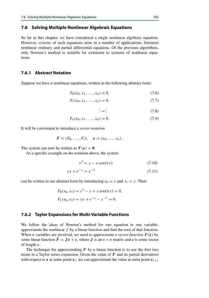
So far in this chapter, we have considered a single nonlinear algebraic equation.
However, systems of such equations arise in a number of applications, foremost
nonlinear ordinary and partial differential equations. Of the previous algorithms,
only Newton’s method is suitable for extension to systems of nonlinear equations.
7.6.1 Abstract Notation
Suppose we have n nonlinear equations, written in the following abstract form:
F 0 (x 0 , x 1 , . . . , x n ) = 0,
(7.6)
F 1 (x 0 , x 1 , . . . , x n ) = 0,
(7.7)
. . . =
. . .
(7.8)
F n (x 0 , x 1 , . . . , x n ) = 0 .
(7.9)
It will be convenient to introduce a vector notation
F = (F 0 , . . . , F 1 ), x = (x 0 , . . . , x n ) .
The system can now be written as F (x) = 0.
As a specific example on the notation above, the system
x
2
= y − x cos(πx)
(7.10)
yx + e
−y
= x
−1
(7.11)
can be written in our abstract form by introducing x 0 = x and x 1 = y. Then
F 0 (x 0 , x 1 ) = x
2
− y + x cos(πx) = 0,
F 1 (x 0 , x 1 ) = yx + e
−y
− x
−1
= 0 .
7.6.2 Taylor Expansions for Multi-Variable Functions
We follow the ideas of Newton’s method for one equation in one variable:
approximate the nonlinear f by a linear function and find the root of that function.
When n variables are involved, we need to approximate a vector function F (x) by
some linear function ˜
F = J x + c, where J is an n × n matrix and c is some vector
of length n.
The technique for approximating F by a linear function is to use the first two
terms in a Taylor series expansion. Given the value of F and its partial derivatives
with respect to x at some point x i , we can approximate the value at some point x i+1
195
7.6 Solving Multiple Nonlinear Algebraic Equations
So far in this chapter, we have considered a single nonlinear algebraic equation.
However, systems of such equations arise in a number of applications, foremost
nonlinear ordinary and partial differential equations. Of the previous algorithms,
only Newton’s method is suitable for extension to systems of nonlinear equations.
7.6.1 Abstract Notation
Suppose we have n nonlinear equations, written in the following abstract form:
F 0 (x 0 , x 1 , . . . , x n ) = 0,
(7.6)
F 1 (x 0 , x 1 , . . . , x n ) = 0,
(7.7)
. . . =
. . .
(7.8)
F n (x 0 , x 1 , . . . , x n ) = 0 .
(7.9)
It will be convenient to introduce a vector notation
F = (F 0 , . . . , F 1 ), x = (x 0 , . . . , x n ) .
The system can now be written as F (x) = 0.
As a specific example on the notation above, the system
x
2
= y − x cos(πx)
(7.10)
yx + e
−y
= x
−1
(7.11)
can be written in our abstract form by introducing x 0 = x and x 1 = y. Then
F 0 (x 0 , x 1 ) = x
2
− y + x cos(πx) = 0,
F 1 (x 0 , x 1 ) = yx + e
−y
− x
−1
= 0 .
7.6.2 Taylor Expansions for Multi-Variable Functions
We follow the ideas of Newton’s method for one equation in one variable:
approximate the nonlinear f by a linear function and find the root of that function.
When n variables are involved, we need to approximate a vector function F (x) by
some linear function ˜
F = J x + c, where J is an n × n matrix and c is some vector
of length n.
The technique for approximating F by a linear function is to use the first two
terms in a Taylor series expansion. Given the value of F and its partial derivatives
with respect to x at some point x i , we can approximate the value at some point x i+1