

184
7 Solving Nonlinear Algebraic Equations
Why Not Use an Array for the x Approximations?
Newton’s method is normally formulated with an iteration index n,
x n+1 = x n −
f (x n )
f (x n )
.
Seeing such an index, many would implement this as
x[n+1] = x[n] - f(x[n])/dfdx(x[n])
Such an array is fine, but requires storage of all the approximations. In large
industrial applications, where Newton’s method solves millions of equations
at once, one cannot afford to store all the intermediate approximations in
memory, so then it is important to understand that the algorithm in Newton’s
method has no more need for x n when x n+1 is computed. Therefore, we can
work with one variable x and overwrite the previous value:
x = x - f(x)/dfdx(x)
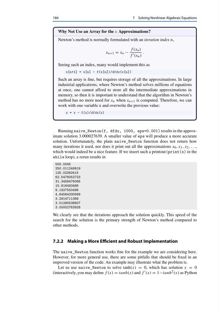
Running naive_Newton(f, dfdx, 1000, eps=0.001) results in the approximate solution 3.000027639. A smaller value of eps will produce a more accurate
solution. Unfortunately, the plain naive_Newton function does not return how
many iterations it used, nor does it print out all the approximations x 0 , x 1 , x 2 , . . .,
which would indeed be a nice feature. If we insert such a printout (print(x) in the
while loop), a rerun results in
500.0045
250.011249919
125.02362415
62.5478052723
31.3458476066
15.816483488
8.1927550496
4.64564330569
3.2914711388
3.01290538807
3.00002763928
We clearly see that the iterations approach the solution quickly. This speed of the
search for the solution is the primary strength of Newton’s method compared to
other methods.
7.2.2 Making a More Efficient and Robust Implementation
The naive_Newton function works fine for the example we are considering here.
However, for more general use, there are some pitfalls that should be fixed in an
improved version of the code. An example may illustrate what the problem is.
Let us use naive_Newton to solve tanh(x) = 0, which has solution x = 0
(interactively, you may define f (x) = tanh(x) and f (x) = 1−tanh 2 (x) as Python
7 Solving Nonlinear Algebraic Equations
Why Not Use an Array for the x Approximations?
Newton’s method is normally formulated with an iteration index n,
x n+1 = x n −
f (x n )
f (x n )
.
Seeing such an index, many would implement this as
x[n+1] = x[n] - f(x[n])/dfdx(x[n])
Such an array is fine, but requires storage of all the approximations. In large
industrial applications, where Newton’s method solves millions of equations
at once, one cannot afford to store all the intermediate approximations in
memory, so then it is important to understand that the algorithm in Newton’s
method has no more need for x n when x n+1 is computed. Therefore, we can
work with one variable x and overwrite the previous value:
x = x - f(x)/dfdx(x)
Running naive_Newton(f, dfdx, 1000, eps=0.001) results in the approximate solution 3.000027639. A smaller value of eps will produce a more accurate
solution. Unfortunately, the plain naive_Newton function does not return how
many iterations it used, nor does it print out all the approximations x 0 , x 1 , x 2 , . . .,
which would indeed be a nice feature. If we insert such a printout (print(x) in the
while loop), a rerun results in
500.0045
250.011249919
125.02362415
62.5478052723
31.3458476066
15.816483488
8.1927550496
4.64564330569
3.2914711388
3.01290538807
3.00002763928
We clearly see that the iterations approach the solution quickly. This speed of the
search for the solution is the primary strength of Newton’s method compared to
other methods.
7.2.2 Making a More Efficient and Robust Implementation
The naive_Newton function works fine for the example we are considering here.
However, for more general use, there are some pitfalls that should be fixed in an
improved version of the code. An example may illustrate what the problem is.
Let us use naive_Newton to solve tanh(x) = 0, which has solution x = 0
(interactively, you may define f (x) = tanh(x) and f (x) = 1−tanh 2 (x) as Python