

6.7 Double and Triple Integrals
163
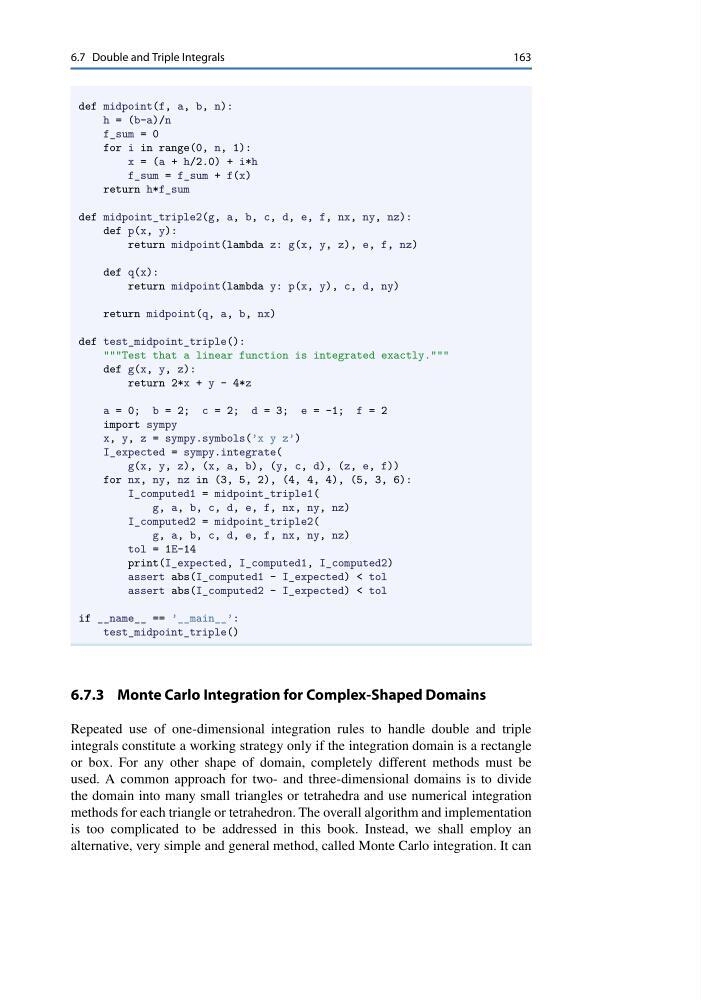
def midpoint(f, a, b, n):
h = (b-a)/n
f_sum = 0
for i in range(0, n, 1):
x = (a + h/2.0) + i*h
f_sum = f_sum + f(x)
return h*f_sum
def midpoint_triple2(g, a, b, c, d, e, f, nx, ny, nz):
def p(x, y):
return midpoint(lambda z: g(x, y, z), e, f, nz)
def q(x):
return midpoint(lambda y: p(x, y), c, d, ny)
return midpoint(q, a, b, nx)
def test_midpoint_triple():
"""Test that a linear function is integrated exactly."""
def g(x, y, z):
return 2*x + y - 4*z
a = 0; b = 2; c = 2; d = 3; e = -1; f = 2
import sympy
x, y, z = sympy.symbols(’x y z’)
I_expected = sympy.integrate(
g(x, y, z), (x, a, b), (y, c, d), (z, e, f))
for nx, ny, nz in (3, 5, 2), (4, 4, 4), (5, 3, 6):
I_computed1 = midpoint_triple1(
g, a, b, c, d, e, f, nx, ny, nz)
I_computed2 = midpoint_triple2(
g, a, b, c, d, e, f, nx, ny, nz)
tol = 1E-14
print(I_expected, I_computed1, I_computed2)
assert abs(I_computed1 - I_expected) < tol
assert abs(I_computed2 - I_expected) < tol
if __name__ == ’__main__’:
test_midpoint_triple()
6.7.3 Monte Carlo Integration for Complex-Shaped Domains
Repeated use of one-dimensional integration rules to handle double and triple
integrals constitute a working strategy only if the integration domain is a rectangle
or box. For any other shape of domain, completely different methods must be
used. A common approach for two- and three-dimensional domains is to divide
the domain into many small triangles or tetrahedra and use numerical integration
methods for each triangle or tetrahedron. The overall algorithm and implementation
is too complicated to be addressed in this book. Instead, we shall employ an
alternative, very simple and general method, called Monte Carlo integration. It can
163
def midpoint(f, a, b, n):
h = (b-a)/n
f_sum = 0
for i in range(0, n, 1):
x = (a + h/2.0) + i*h
f_sum = f_sum + f(x)
return h*f_sum
def midpoint_triple2(g, a, b, c, d, e, f, nx, ny, nz):
def p(x, y):
return midpoint(lambda z: g(x, y, z), e, f, nz)
def q(x):
return midpoint(lambda y: p(x, y), c, d, ny)
return midpoint(q, a, b, nx)
def test_midpoint_triple():
"""Test that a linear function is integrated exactly."""
def g(x, y, z):
return 2*x + y - 4*z
a = 0; b = 2; c = 2; d = 3; e = -1; f = 2
import sympy
x, y, z = sympy.symbols(’x y z’)
I_expected = sympy.integrate(
g(x, y, z), (x, a, b), (y, c, d), (z, e, f))
for nx, ny, nz in (3, 5, 2), (4, 4, 4), (5, 3, 6):
I_computed1 = midpoint_triple1(
g, a, b, c, d, e, f, nx, ny, nz)
I_computed2 = midpoint_triple2(
g, a, b, c, d, e, f, nx, ny, nz)
tol = 1E-14
print(I_expected, I_computed1, I_computed2)
assert abs(I_computed1 - I_expected) < tol
assert abs(I_computed2 - I_expected) < tol
if __name__ == ’__main__’:
test_midpoint_triple()
6.7.3 Monte Carlo Integration for Complex-Shaped Domains
Repeated use of one-dimensional integration rules to handle double and triple
integrals constitute a working strategy only if the integration domain is a rectangle
or box. For any other shape of domain, completely different methods must be
used. A common approach for two- and three-dimensional domains is to divide
the domain into many small triangles or tetrahedra and use numerical integration
methods for each triangle or tetrahedron. The overall algorithm and implementation
is too complicated to be addressed in this book. Instead, we shall employ an
alternative, very simple and general method, called Monte Carlo integration. It can