

148
6 Computing Integrals and Testing Code
6.4.3 Speed up Gained with Vectorization
Now that we have created faster, vectorized versions of the functions, it is of interest
to measure how much faster they are. Restricting ourselves to the midpoint method,
we might proceed as:
import timeit
from integration_methods_vec import midpoint as midpoint_vec
from midpoint import midpoint
from numpy import exp
v = lambda t: 3*t**2*exp(t**3)
t = timeit.Timer(’midpoint(v, 0, 1, 1000000)’, \
setup=’from __main__ import midpoint, v’)
time_midpoint = t.timeit(10)
print(’Time, midpoint: {:g} seconds’.format(time_midpoint))
# Vectorized version
t = timeit.Timer(’midpoint_vec(v, 0, 1, 1000000)’, \
setup=’from __main__ import midpoint_vec, v’)
time_midpoint_vec = t.timeit(10)
print(’Time, midpoint vec: {:g} seconds’.format(time_midpoint_vec))
print(’Efficiency factor: {:g}’.format(time_midpoint/time_midpoint_vec))
Running the program gives
Time, midpoint: 19.6083 seconds
Time, midpoint vec: 0.868379 seconds
Efficiency factor: 22.5804
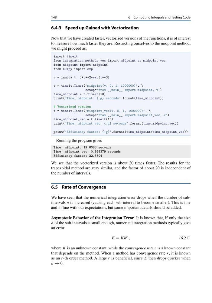
We see that the vectorized version is about 20 times faster. The results for the
trapezoidal method are very similar, and the factor of about 20 is independent of
the number of intervals.
6.5 Rate of Convergence
We have seen that the numerical integration error drops when the number of subintervals n is increased (causing each sub-interval to become smaller). This is fine
and in line with our expectations, but some important details should be added.
Asymptotic Behavior of the Integration Error It is known that, if only the size
h of the sub-intervals is small enough, numerical integration methods typically give
an error
E = Kh
r ,
(6.21)
where K is an unknown constant, while the convergence rate r is a known constant
that depends on the method. When a method has convergence rate r, it is known
as an r-th order method. A large r is beneficial, since E then drops quicker when
h → 0.
6 Computing Integrals and Testing Code
6.4.3 Speed up Gained with Vectorization
Now that we have created faster, vectorized versions of the functions, it is of interest
to measure how much faster they are. Restricting ourselves to the midpoint method,
we might proceed as:
import timeit
from integration_methods_vec import midpoint as midpoint_vec
from midpoint import midpoint
from numpy import exp
v = lambda t: 3*t**2*exp(t**3)
t = timeit.Timer(’midpoint(v, 0, 1, 1000000)’, \
setup=’from __main__ import midpoint, v’)
time_midpoint = t.timeit(10)
print(’Time, midpoint: {:g} seconds’.format(time_midpoint))
# Vectorized version
t = timeit.Timer(’midpoint_vec(v, 0, 1, 1000000)’, \
setup=’from __main__ import midpoint_vec, v’)
time_midpoint_vec = t.timeit(10)
print(’Time, midpoint vec: {:g} seconds’.format(time_midpoint_vec))
print(’Efficiency factor: {:g}’.format(time_midpoint/time_midpoint_vec))
Running the program gives
Time, midpoint: 19.6083 seconds
Time, midpoint vec: 0.868379 seconds
Efficiency factor: 22.5804
We see that the vectorized version is about 20 times faster. The results for the
trapezoidal method are very similar, and the factor of about 20 is independent of
the number of intervals.
6.5 Rate of Convergence
We have seen that the numerical integration error drops when the number of subintervals n is increased (causing each sub-interval to become smaller). This is fine
and in line with our expectations, but some important details should be added.
Asymptotic Behavior of the Integration Error It is known that, if only the size
h of the sub-intervals is small enough, numerical integration methods typically give
an error
E = Kh
r ,
(6.21)
where K is an unknown constant, while the convergence rate r is a known constant
that depends on the method. When a method has convergence rate r, it is known
as an r-th order method. A large r is beneficial, since E then drops quicker when
h → 0.