

136
6 Computing Integrals and Testing Code
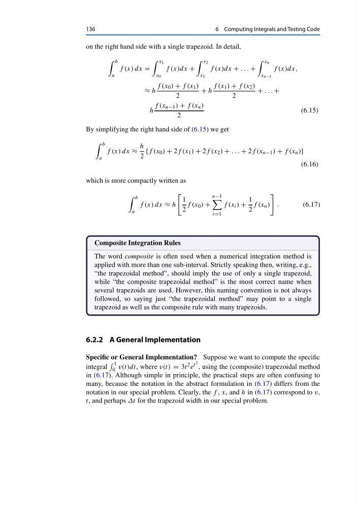
on the right hand side with a single trapezoid. In detail,
b
a
f (x) dx =
x 1
x 0
f (x)dx +
x 2
x 1
f (x)dx + . . . +
x n
x n−1
f (x)dx,
≈ h
f (x 0 ) + f (x 1 )
2
+ h
f (x 1 ) + f (x 2 )
2
+ . . . +
h
f (x n−1 ) + f (x n )
2
(6.15)
By simplifying the right hand side of (6.15) we get
b
a
f (x) dx ≈
h
2
[f (x 0 ) + 2f (x 1 ) + 2f (x 2 ) + . . . + 2f (x n−1 ) + f (x n )]
(6.16)
which is more compactly written as
b
a
f (x) dx ≈ h
1
2
f (x 0 ) +
n−1
i=1
f (x i ) +
1
2
f (x n )
.
(6.17)
Composite Integration Rules
The word composite is often used when a numerical integration method is
applied with more than one sub-interval. Strictly speaking then, writing, e.g.,
“the trapezoidal method”, should imply the use of only a single trapezoid,
while “the composite trapezoidal method” is the most correct name when
several trapezoids are used. However, this naming convention is not always
followed, so saying just “the trapezoidal method” may point to a single
trapezoid as well as the composite rule with many trapezoids.
6.2.2 A General Implementation
Specific or General Implementation? Suppose we want to compute the specific
integral
1
0 v(t)dt, where v(t) = 3t 2 e t 3 , using the (composite) trapezoidal method
in (6.17). Although simple in principle, the practical steps are often confusing to
many, because the notation in the abstract formulation in (6.17) differs from the
notation in our special problem. Clearly, the f , x, and h in (6.17) correspond to v,
t, and perhaps Δt for the trapezoid width in our special problem.
6 Computing Integrals and Testing Code
on the right hand side with a single trapezoid. In detail,
b
a
f (x) dx =
x 1
x 0
f (x)dx +
x 2
x 1
f (x)dx + . . . +
x n
x n−1
f (x)dx,
≈ h
f (x 0 ) + f (x 1 )
2
+ h
f (x 1 ) + f (x 2 )
2
+ . . . +
h
f (x n−1 ) + f (x n )
2
(6.15)
By simplifying the right hand side of (6.15) we get
b
a
f (x) dx ≈
h
2
[f (x 0 ) + 2f (x 1 ) + 2f (x 2 ) + . . . + 2f (x n−1 ) + f (x n )]
(6.16)
which is more compactly written as
b
a
f (x) dx ≈ h
1
2
f (x 0 ) +
n−1
i=1
f (x i ) +
1
2
f (x n )
.
(6.17)
Composite Integration Rules
The word composite is often used when a numerical integration method is
applied with more than one sub-interval. Strictly speaking then, writing, e.g.,
“the trapezoidal method”, should imply the use of only a single trapezoid,
while “the composite trapezoidal method” is the most correct name when
several trapezoids are used. However, this naming convention is not always
followed, so saying just “the trapezoidal method” may point to a single
trapezoid as well as the composite rule with many trapezoids.
6.2.2 A General Implementation
Specific or General Implementation? Suppose we want to compute the specific
integral
1
0 v(t)dt, where v(t) = 3t 2 e t 3 , using the (composite) trapezoidal method
in (6.17). Although simple in principle, the practical steps are often confusing to
many, because the notation in the abstract formulation in (6.17) differs from the
notation in our special problem. Clearly, the f , x, and h in (6.17) correspond to v,
t, and perhaps Δt for the trapezoid width in our special problem.