

134
6 Computing Integrals and Testing Code
6.2 The Composite Trapezoidal Rule
The integral
b
a f (x)dx may be interpreted as the area between the x axis and the
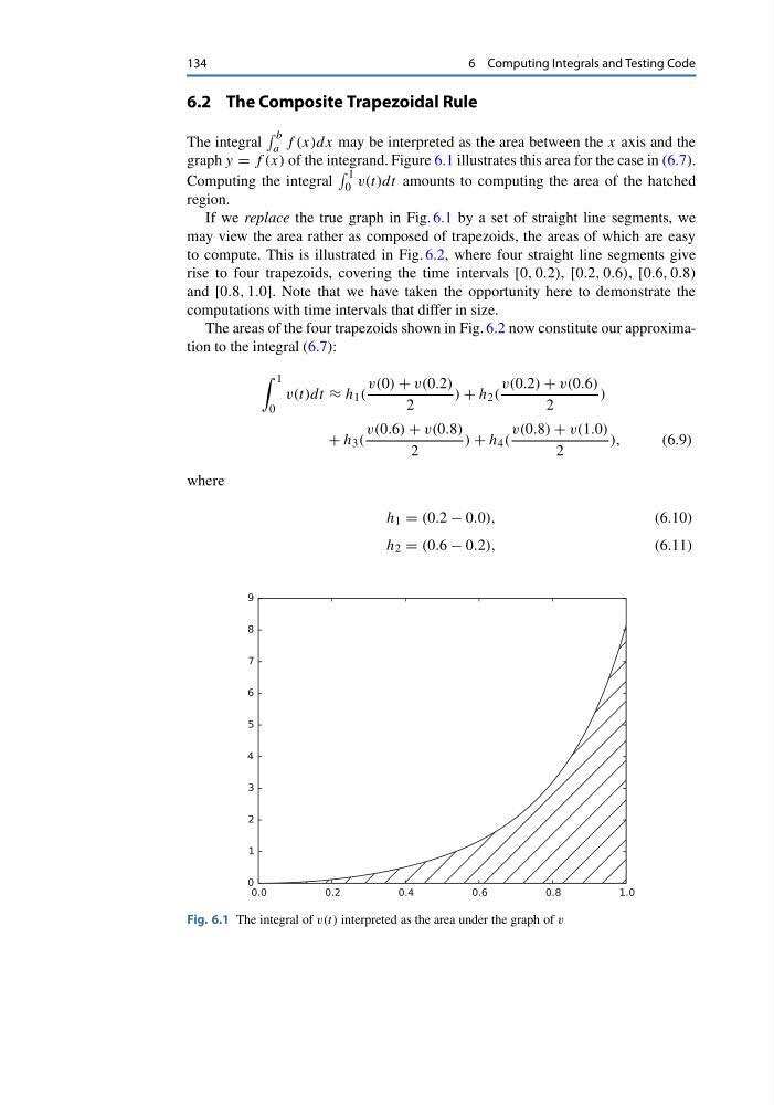
graph y = f (x) of the integrand. Figure 6.1 illustrates this area for the case in (6.7).
Computing the integral
1
0 v(t)dt amounts to computing the area of the hatched
region.
If we replace the true graph in Fig. 6.1 by a set of straight line segments, we
may view the area rather as composed of trapezoids, the areas of which are easy
to compute. This is illustrated in Fig. 6.2, where four straight line segments give
rise to four trapezoids, covering the time intervals [0, 0.2), [0.2, 0.6), [0.6, 0.8)
and [0.8, 1.0]. Note that we have taken the opportunity here to demonstrate the
computations with time intervals that differ in size.
The areas of the four trapezoids shown in Fig. 6.2 now constitute our approximation to the integral (6.7):
1
0
v(t)dt ≈ h 1 (
v(0) + v(0.2)
2
) + h 2 (
v(0.2) + v(0.6)
2
)
+ h 3 (
v(0.6) + v(0.8)
2
) + h 4 (
v(0.8) + v(1.0)
2
),
(6.9)
where
h 1 = (0.2 − 0.0),
(6.10)
h 2 = (0.6 − 0.2),
(6.11)
Fig. 6.1 The integral of v(t) interpreted as the area under the graph of v
6 Computing Integrals and Testing Code
6.2 The Composite Trapezoidal Rule
The integral
b
a f (x)dx may be interpreted as the area between the x axis and the
graph y = f (x) of the integrand. Figure 6.1 illustrates this area for the case in (6.7).
Computing the integral
1
0 v(t)dt amounts to computing the area of the hatched
region.
If we replace the true graph in Fig. 6.1 by a set of straight line segments, we
may view the area rather as composed of trapezoids, the areas of which are easy
to compute. This is illustrated in Fig. 6.2, where four straight line segments give
rise to four trapezoids, covering the time intervals [0, 0.2), [0.2, 0.6), [0.6, 0.8)
and [0.8, 1.0]. Note that we have taken the opportunity here to demonstrate the
computations with time intervals that differ in size.
The areas of the four trapezoids shown in Fig. 6.2 now constitute our approximation to the integral (6.7):
1
0
v(t)dt ≈ h 1 (
v(0) + v(0.2)
2
) + h 2 (
v(0.2) + v(0.6)
2
)
+ h 3 (
v(0.6) + v(0.8)
2
) + h 4 (
v(0.8) + v(1.0)
2
),
(6.9)
where
h 1 = (0.2 − 0.0),
(6.10)
h 2 = (0.6 − 0.2),
(6.11)
Fig. 6.1 The integral of v(t) interpreted as the area under the graph of v