

72
F. Frohn
LoAT Monot. Meter Flata
exact 1444 845
0
3
1231
approx 38
0
733
0
fail
29
666
778 280
avg rt 0.16s 0.11s 0.09s 0.47s
Table 1.
Ev-Inc Ev-Dec Ev-Mon
exact 1444
845
845
approx
0
493
0
fail
67
173
666
avg rt 0.15s 0.14s
0.09s
Table 2.
LoAT:
Acceleration calculus + Theorems 7, 8, 11 and 13
Monot.: Acceleration via Monotonicity, Thm. 3
Meter: Acceleration via Metering Functions, Thm. 4
Flata:
The tool Flata, see http://nts.imag.fr/index.php/Flata
Ev-Inc: Acceleration calculus + Theorems 7, 8 and 11
Ev-Dec: Acceleration calculus + Theorems 7, 8 and 13
Ev-Mon: Acceleration calculus + Theorems 7 and 8
exact:
Number of examples that were accelerated exactly
approx: Number of examples that were accelerated approximately
fail:
Number of examples that could not be accelerated
avg rt: Average runtime per example
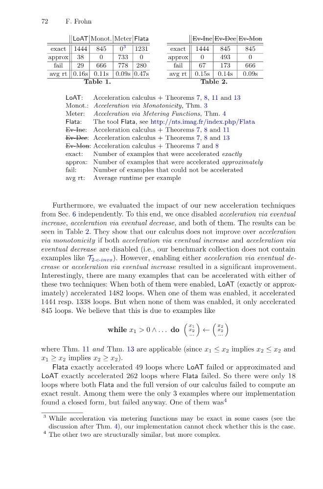
Furthermore, we evaluated the impact of our new acceleration techniques
from Sec. 6 independently. To this end, we once disabled acceleration via eventual
increase, acceleration via eventual decrease, and both of them. The results can be
seen in Table 2. They show that our calculus does not improve over acceleration
via monotonicity if both acceleration via eventual increase and acceleration via
eventual decrease are disabled (i.e., our benchmark collection does not contain
examples like T 2-c-invs ). However, enabling either acceleration via eventual decrease or acceleration via eventual increase resulted in a significant improvement.
Interestingly, there are many examples that can be accelerated with either of
these two techniques: When both of them were enabled, LoAT (exactly or approximately) accelerated 1482 loops. When one of them was enabled, it accelerated
1444 resp. 1338 loops. But when none of them was enabled, it only accelerated
845 loops. We believe that this is due to examples like
while x 1 > 0 ∧ . . . do
x1
x2
...
←
x2
x2
...
where Thm. 11 and Thm. 13 are applicable (since x 1 ≤ x 2 implies x 2 ≤ x 2 and
x 1 ≥ x 2 implies x 2 ≥ x 2 ).
Flata exactly accelerated 49 loops where LoAT failed or approximated and
LoAT exactly accelerated 262 loops where Flata failed. So there were only 18
loops where both Flata and the full version of our calculus failed to compute an
exact result. Among them were the only 3 examples where our implementation
found a closed form, but failed anyway. One of them was
4
3 While acceleration via metering functions may be exact in some cases (see the
discussion after Thm. 4), our implementation cannot check whether this is the case.
4 The other two are structurally similar, but more complex.
F. Frohn
LoAT Monot. Meter Flata
exact 1444 845
0
3
1231
approx 38
0
733
0
fail
29
666
778 280
avg rt 0.16s 0.11s 0.09s 0.47s
Table 1.
Ev-Inc Ev-Dec Ev-Mon
exact 1444
845
845
approx
0
493
0
fail
67
173
666
avg rt 0.15s 0.14s
0.09s
Table 2.
LoAT:
Acceleration calculus + Theorems 7, 8, 11 and 13
Monot.: Acceleration via Monotonicity, Thm. 3
Meter: Acceleration via Metering Functions, Thm. 4
Flata:
The tool Flata, see http://nts.imag.fr/index.php/Flata
Ev-Inc: Acceleration calculus + Theorems 7, 8 and 11
Ev-Dec: Acceleration calculus + Theorems 7, 8 and 13
Ev-Mon: Acceleration calculus + Theorems 7 and 8
exact:
Number of examples that were accelerated exactly
approx: Number of examples that were accelerated approximately
fail:
Number of examples that could not be accelerated
avg rt: Average runtime per example
Furthermore, we evaluated the impact of our new acceleration techniques
from Sec. 6 independently. To this end, we once disabled acceleration via eventual
increase, acceleration via eventual decrease, and both of them. The results can be
seen in Table 2. They show that our calculus does not improve over acceleration
via monotonicity if both acceleration via eventual increase and acceleration via
eventual decrease are disabled (i.e., our benchmark collection does not contain
examples like T 2-c-invs ). However, enabling either acceleration via eventual decrease or acceleration via eventual increase resulted in a significant improvement.
Interestingly, there are many examples that can be accelerated with either of
these two techniques: When both of them were enabled, LoAT (exactly or approximately) accelerated 1482 loops. When one of them was enabled, it accelerated
1444 resp. 1338 loops. But when none of them was enabled, it only accelerated
845 loops. We believe that this is due to examples like
while x 1 > 0 ∧ . . . do
x1
x2
...
←
x2
x2
...
where Thm. 11 and Thm. 13 are applicable (since x 1 ≤ x 2 implies x 2 ≤ x 2 and
x 1 ≥ x 2 implies x 2 ≥ x 2 ).
Flata exactly accelerated 49 loops where LoAT failed or approximated and
LoAT exactly accelerated 262 loops where Flata failed. So there were only 18
loops where both Flata and the full version of our calculus failed to compute an
exact result. Among them were the only 3 examples where our implementation
found a closed form, but failed anyway. One of them was
4
3 While acceleration via metering functions may be exact in some cases (see the
discussion after Thm. 4), our implementation cannot check whether this is the case.
4 The other two are structurally similar, but more complex.