

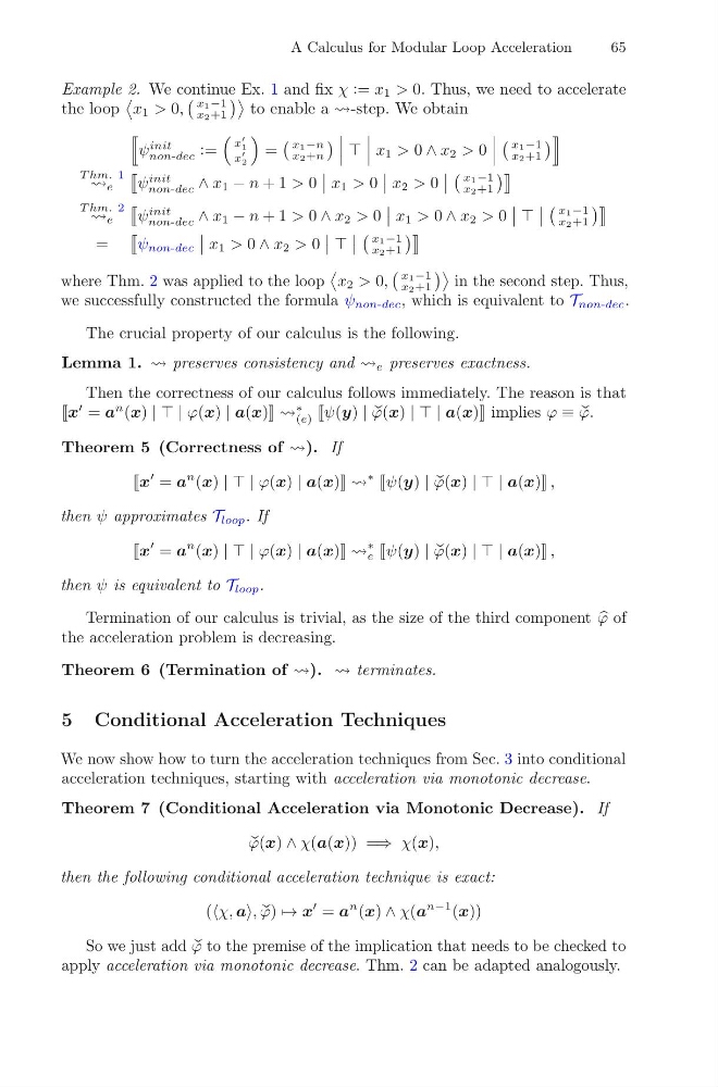
A Calculus for Modular Loop Acceleration
65
Example 2. We continue Ex. 1 and fix χ := x 1 > 0. Thus, we need to accelerate
the loop
x 1 > 0,
x1−1
x2+1
to enable a -step. We obtain
ψ
init
non-dec :=
x
1
x
2
=
x1−n
x2+n
x 1 > 0 ∧ x 2 > 0
x1−1
x2+1
T hm. 1
e
ψ
init
non-dec ∧ x 1 − n + 1 > 0
x 1 > 0
x 2 > 0
x1−1
x2+1
T hm. 2
e
ψ
init
non-dec ∧ x 1 − n + 1 > 0 ∧ x 2 > 0
x 1 > 0 ∧ x 2 > 0
x1−1
x2+1
=
ψ non-dec
x 1 > 0 ∧ x 2 > 0
x1−1
x2+1
where Thm. 2 was applied to the loop
x 2 > 0,
x1−1
x2+1
in the second step. Thus,
we successfully constructed the formula ψ non-dec , which is equivalent to T non-dec .
The crucial property of our calculus is the following.
Lemma 1. preserves consistency and e preserves exactness.
Then the correctness of our calculus follows immediately. The reason is that
x
= a
n (x) | | | ϕ(x) | a(x)
∗
(e) ψ(y) | q
ϕ(x) | | | a(x) implies ϕ ≡ q
ϕ.
Theorem 5 (Correctness of ). If
x
= a
n (x) | | | ϕ(x) | a(x)
∗
ψ(y) | q
ϕ(x) | | | a(x) ,
then ψ approximates T loop . If
x
= a
n (x) | | | ϕ(x) | a(x)
∗
e ψ(y) | q
ϕ(x) | | | a(x) ,
then ψ is equivalent to T loop .
Termination of our calculus is trivial, as the size of the third component
ϕ of
the acceleration problem is decreasing.
Theorem 6 (Termination of ). terminates.
5 Conditional Acceleration Techniques
We now show how to turn the acceleration techniques from Sec. 3 into conditional
acceleration techniques, starting with acceleration via monotonic decrease.
Theorem 7 (Conditional Acceleration via Monotonic Decrease). If
q
ϕ(x) ∧ χ(a(x)) =⇒ χ(x),
then the following conditional acceleration technique is exact:
(χ, a, q
ϕ) → x
= a
n (x) ∧ χ(a
n−1 (x))
So we just add q
ϕ to the premise of the implication that needs to be checked to
apply acceleration via monotonic decrease. Thm. 2 can be adapted analogously.
65
Example 2. We continue Ex. 1 and fix χ := x 1 > 0. Thus, we need to accelerate
the loop
x 1 > 0,
x1−1
x2+1
to enable a -step. We obtain
ψ
init
non-dec :=
x
1
x
2
=
x1−n
x2+n
x 1 > 0 ∧ x 2 > 0
x1−1
x2+1
T hm. 1
e
ψ
init
non-dec ∧ x 1 − n + 1 > 0
x 1 > 0
x 2 > 0
x1−1
x2+1
T hm. 2
e
ψ
init
non-dec ∧ x 1 − n + 1 > 0 ∧ x 2 > 0
x 1 > 0 ∧ x 2 > 0
x1−1
x2+1
=
ψ non-dec
x 1 > 0 ∧ x 2 > 0
x1−1
x2+1
where Thm. 2 was applied to the loop
x 2 > 0,
x1−1
x2+1
in the second step. Thus,
we successfully constructed the formula ψ non-dec , which is equivalent to T non-dec .
The crucial property of our calculus is the following.
Lemma 1. preserves consistency and e preserves exactness.
Then the correctness of our calculus follows immediately. The reason is that
x
= a
n (x) | | | ϕ(x) | a(x)
∗
(e) ψ(y) | q
ϕ(x) | | | a(x) implies ϕ ≡ q
ϕ.
Theorem 5 (Correctness of ). If
x
= a
n (x) | | | ϕ(x) | a(x)
∗
ψ(y) | q
ϕ(x) | | | a(x) ,
then ψ approximates T loop . If
x
= a
n (x) | | | ϕ(x) | a(x)
∗
e ψ(y) | q
ϕ(x) | | | a(x) ,
then ψ is equivalent to T loop .
Termination of our calculus is trivial, as the size of the third component
ϕ of
the acceleration problem is decreasing.
Theorem 6 (Termination of ). terminates.
5 Conditional Acceleration Techniques
We now show how to turn the acceleration techniques from Sec. 3 into conditional
acceleration techniques, starting with acceleration via monotonic decrease.
Theorem 7 (Conditional Acceleration via Monotonic Decrease). If
q
ϕ(x) ∧ χ(a(x)) =⇒ χ(x),
then the following conditional acceleration technique is exact:
(χ, a, q
ϕ) → x
= a
n (x) ∧ χ(a
n−1 (x))
So we just add q
ϕ to the premise of the implication that needs to be checked to
apply acceleration via monotonic decrease. Thm. 2 can be adapted analogously.