

Verifying Array Manipulating Programs with Full-Program Induction
33
Algorithm 5 SimplifyDiff(∂PN : difference program)
1: ∂PN := (Locs, E, μ)
2: ∂P
N := (Locs
, E
, μ
), where Locs
:= Locs, E
:= E, and μ
:= μ;
3: for each loop L ∈ Loops(∂PN ) do
4:
(n1, n, U) := IncomingEdge(L); (n, n2, ff ) := ExitEdge(L);
5:
if Loop body of L is of the form wN := wN op expr, wherein wN is a scalar variable then
6:
nacc = FreshNode();
7:
if op ∈ {+, −} then
8:
μ
(nacc) := (wN := wN op Simplify(kL(N − 1) ∗ expr));
9:
else if op ∈ {∗, ÷} then
10:
μ
(nacc) := (wN := wN op Simplify(expr
k L (N −1) ));
11:
else throw “Specified operator not handled”;
12:
E
:= E
- {(n1, n, U), (n, n2, ff )} ∪ {(n1, nacc, U), (nacc, n2, U)};
13:
Locs
:= Locs
− Nodes(L) ∪ {nacc} ;
14:
if Loop body of L is of the form wN := wNm1 or wN := wN then
15:
E
:= E
− {(n1, n, U), (n, n2, ff )} ∪ {(n1, n2, U)}; Locs
:= Locs
− Nodes(L);
16: return ∂P
N
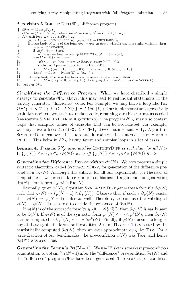
Simplifying the Difference Program. While we have described a simple
strategy to generate ∂P N above, this may lead to redundant statements in the
naively generated “difference” code. For example, we may have a loop like for
(i=0; i < N-1; i++) A N[i] = A Nm1[i];. Our implementation aggressively
optimizes and removes such redundant code, renaming variables/arrays as needed
(see routine SimplifyDiff in Algorithm 5). The program ∂P N may also contain
loops that compute values of variables that can be accelerated. For example,
we may have a loop for(i=0; i < N-1; i++) sum = sum + 1;. Algorithm
SimplifyDiff removes this loop and introduces the statement sum = sum +
(N-1);. This helps in ∂P N having fewer and simpler loops in a lot of cases.
Lemma 4. Program ∂P
N generated by SimplifyDiff is such that, for all N >
1, {ϕ(N )} P N −1 ; ∂P
N {ψ(N )} holds iff {ϕ(N )} P N −1 ; ∂P N {ψ(N )} holds.
Generating the Difference Pre-condition ∂ϕ(N). We now present a simple
syntactic algorithm, called SyntacticDiff, for generation of the difference precondition ∂ϕ(N ). Although this suffices for all our experiments, for the sake of
completeness, we present later a more sophisticated algorithm for generating
∂ϕ(N ) simultaneously with Pre(N ).
Formally, given ϕ(N ), algorithm SyntacticDiff generates a formula ∂ϕ(N )
such that ϕ(N ) → (ϕ(N − 1) ∧ ∂ϕ(N )). Observe that if such a ∂ϕ(N ) exists,
then ϕ(N ) → ϕ(N − 1) holds as well. Therefore, we can use the validity of
ϕ(N ) → ϕ(N − 1) as a test to decide the existence of ∂ϕ(N ).
If ϕ(N ) is of the syntactic form ∀i ∈ {0 . . . N}
ϕ(i), then ∂ϕ(N ) is easily seen
to be ˆ
ϕ(N ). If ϕ(N ) is of the syntactic form ϕ
1 (N ) ∧ · · · ∧ ϕ
k (N ), then ∂ϕ(N )
can be computed as ∂ϕ
1 (N ) ∧ · · · ∧ ∂ϕ
k (N ). Finally, if ϕ(N ) doesn’t belong to
any of these syntactic forms or if condition 2(a) of Theorem 1 is violated by the
heuristically computed ∂ϕ(N ), then we over-approximate ∂ϕ N by True. For a
large fraction of our benchmarks, the pre-condition ϕ(N ) was True, and hence
∂ϕ(N ) was also True.
Generating the Formula Pre(N − 1). We use Dijsktra’s weakest pre-condition
computation to obtain Pre(N −1) after the “difference” pre-condition ∂ϕ(N ) and
the “difference” program ∂P N have been generated. The weakest pre-condition
33
Algorithm 5 SimplifyDiff(∂PN : difference program)
1: ∂PN := (Locs, E, μ)
2: ∂P
N := (Locs
, E
, μ
), where Locs
:= Locs, E
:= E, and μ
:= μ;
3: for each loop L ∈ Loops(∂PN ) do
4:
(n1, n, U) := IncomingEdge(L); (n, n2, ff ) := ExitEdge(L);
5:
if Loop body of L is of the form wN := wN op expr, wherein wN is a scalar variable then
6:
nacc = FreshNode();
7:
if op ∈ {+, −} then
8:
μ
(nacc) := (wN := wN op Simplify(kL(N − 1) ∗ expr));
9:
else if op ∈ {∗, ÷} then
10:
μ
(nacc) := (wN := wN op Simplify(expr
k L (N −1) ));
11:
else throw “Specified operator not handled”;
12:
E
:= E
- {(n1, n, U), (n, n2, ff )} ∪ {(n1, nacc, U), (nacc, n2, U)};
13:
Locs
:= Locs
− Nodes(L) ∪ {nacc} ;
14:
if Loop body of L is of the form wN := wNm1 or wN := wN then
15:
E
:= E
− {(n1, n, U), (n, n2, ff )} ∪ {(n1, n2, U)}; Locs
:= Locs
− Nodes(L);
16: return ∂P
N
Simplifying the Difference Program. While we have described a simple
strategy to generate ∂P N above, this may lead to redundant statements in the
naively generated “difference” code. For example, we may have a loop like for
(i=0; i < N-1; i++) A N[i] = A Nm1[i];. Our implementation aggressively
optimizes and removes such redundant code, renaming variables/arrays as needed
(see routine SimplifyDiff in Algorithm 5). The program ∂P N may also contain
loops that compute values of variables that can be accelerated. For example,
we may have a loop for(i=0; i < N-1; i++) sum = sum + 1;. Algorithm
SimplifyDiff removes this loop and introduces the statement sum = sum +
(N-1);. This helps in ∂P N having fewer and simpler loops in a lot of cases.
Lemma 4. Program ∂P
N generated by SimplifyDiff is such that, for all N >
1, {ϕ(N )} P N −1 ; ∂P
N {ψ(N )} holds iff {ϕ(N )} P N −1 ; ∂P N {ψ(N )} holds.
Generating the Difference Pre-condition ∂ϕ(N). We now present a simple
syntactic algorithm, called SyntacticDiff, for generation of the difference precondition ∂ϕ(N ). Although this suffices for all our experiments, for the sake of
completeness, we present later a more sophisticated algorithm for generating
∂ϕ(N ) simultaneously with Pre(N ).
Formally, given ϕ(N ), algorithm SyntacticDiff generates a formula ∂ϕ(N )
such that ϕ(N ) → (ϕ(N − 1) ∧ ∂ϕ(N )). Observe that if such a ∂ϕ(N ) exists,
then ϕ(N ) → ϕ(N − 1) holds as well. Therefore, we can use the validity of
ϕ(N ) → ϕ(N − 1) as a test to decide the existence of ∂ϕ(N ).
If ϕ(N ) is of the syntactic form ∀i ∈ {0 . . . N}
ϕ(i), then ∂ϕ(N ) is easily seen
to be ˆ
ϕ(N ). If ϕ(N ) is of the syntactic form ϕ
1 (N ) ∧ · · · ∧ ϕ
k (N ), then ∂ϕ(N )
can be computed as ∂ϕ
1 (N ) ∧ · · · ∧ ∂ϕ
k (N ). Finally, if ϕ(N ) doesn’t belong to
any of these syntactic forms or if condition 2(a) of Theorem 1 is violated by the
heuristically computed ∂ϕ(N ), then we over-approximate ∂ϕ N by True. For a
large fraction of our benchmarks, the pre-condition ϕ(N ) was True, and hence
∂ϕ(N ) was also True.
Generating the Formula Pre(N − 1). We use Dijsktra’s weakest pre-condition
computation to obtain Pre(N −1) after the “difference” pre-condition ∂ϕ(N ) and
the “difference” program ∂P N have been generated. The weakest pre-condition