

Learning One-Clock Timed Automata
451
T5
−
(a, 1.1, ⊥) +
(a, 0, −
(b, 0, −
(a, 1.1, ⊥)(a, 0, −
(a, 1.1, ⊥)(b, 0, −
(a, 1.1, ⊥)(b, 2, +
(a, 3, −
q−
start
q+
(a, 0,
(a, 3,
(b, 0,
(a, 1.1, ⊥)
(b, 2,
(a, 0,
(b, 0,
M5
q−
start
q+
a, [0, 1],
a, [3, ∞),
b, [0, ∞),
a, (1, 3), ⊥
b, [2, ∞),
a, [0, ∞),
b, [0, 2),
H5
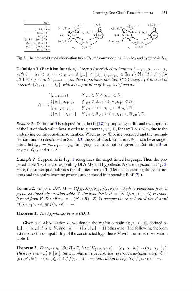
Fig. 2: The prepared timed observation table T5, the corresponding DFA M5 and hypothesis H5.
Definition 3 (Partition function). Given a list of clock valuations = μ 0 , μ 1 , · · · , μ n
with 0 = μ 0 < μ 1 · · · < μ n , and i = j if μ i , μ j ∈ R ≥0 \ N and i = j for
all 1 ≤ i, j ≤ n, let μ n+1 = ∞, then a partition function P
c
(·) mapping to a set of
intervals {I 0 , I 1 , . . . , I n }, which is a partition of R ≥0 , is defined as
I i =
⎧
⎪ ⎪ ⎪ ⎨
⎪ ⎪ ⎪ ⎩
[μ i , μ i+1 ),
if μ i ∈ N ∧ μ i+1 ∈ N;
( i , μ i+1 ),
if μ i ∈ R ≥0 \ N ∧ μ i+1 ∈ N;
[μ i , i+1
if μ i ∈ N ∧ μ i+1 ∈ R ≥0 \ N;
( i i+1 if μ i ∈ R ≥0 \ N ∧ μ i+1 ∈ R ≥0 \ N.
Remark 2. Definition 3 is adapted from that in [18] by imposing additional assumptions
of the list of clock valuations in order to guarantee μ i ∈ I i , for any 0 ≤ i ≤ n, due to the
underlying continuous-time semantics. Whereas, by T being prepared and the normalization function described in Sect. 3.3, the set of clock valuations Ψ q,σ can be arranged
into a list q,σ = μ 0 , μ 1 , . . . , μ n satisfying such assumptions given in Definition 3 for
any q ∈ Q M and σ ∈ Σ.
Example 2. Suppose A in Fig. 1 recognizes the target timed language. Then the prepared table T 5 , the corresponding DFA M 5 and hypothesis H 5 are depicted in Fig. 2.
Here, the subscript 5 indicates the fifth iteration of T (Details concerning the constructions and the entire learning process are enclosed in Appendix B of [7].).
Lemma 2. Given a DFA M = (Q M , Σ M , δ M , q
0
M , F M ), which is generated from a
prepared timed observation table T, the hypothesis H = (Σ, Q, q 0 , F, c, Δ) is transformed from M. For all γ r · e ∈ (S ∪ R) · E, H accepts the reset-logical-timed word
π(Π {1,2} γ r · e) iff f (γ r · e) = +.
Theorem 2. The hypothesis H is a COTA.
Given a clock valuation μ, we denote the region containing μ as defined as
= [μ, μ] if μ ∈ N, and = ( + 1) otherwise. The following theorem
establishes the compatibility of the constructed hypothesis H with the timed observation
table T.
Theorem 3. For γ r ·e ∈ (S ∪R)·E, let π(Π {1,2} γ r ·e) = (σ 1 , μ 1 , b 1 ) · · · (σ n , μ n , b n ).
Then for every μ
i ∈ i , the hypothesis H accepts the reset-logical-timed word γ
r =
(σ 1 , μ
1 , b 1 ) · · · (σ n , μ
n , b n ) if f (γ r · e) = +, and cannot accept it if f (γ r · e) = −.
451
T5
−
(a, 1.1, ⊥) +
(a, 0, −
(b, 0, −
(a, 1.1, ⊥)(a, 0, −
(a, 1.1, ⊥)(b, 0, −
(a, 1.1, ⊥)(b, 2, +
(a, 3, −
q−
start
q+
(a, 0,
(a, 3,
(b, 0,
(a, 1.1, ⊥)
(b, 2,
(a, 0,
(b, 0,
M5
q−
start
q+
a, [0, 1],
a, [3, ∞),
b, [0, ∞),
a, (1, 3), ⊥
b, [2, ∞),
a, [0, ∞),
b, [0, 2),
H5
Fig. 2: The prepared timed observation table T5, the corresponding DFA M5 and hypothesis H5.
Definition 3 (Partition function). Given a list of clock valuations = μ 0 , μ 1 , · · · , μ n
with 0 = μ 0 < μ 1 · · · < μ n , and i = j if μ i , μ j ∈ R ≥0 \ N and i = j for
all 1 ≤ i, j ≤ n, let μ n+1 = ∞, then a partition function P
c
(·) mapping to a set of
intervals {I 0 , I 1 , . . . , I n }, which is a partition of R ≥0 , is defined as
I i =
⎧
⎪ ⎪ ⎪ ⎨
⎪ ⎪ ⎪ ⎩
[μ i , μ i+1 ),
if μ i ∈ N ∧ μ i+1 ∈ N;
( i , μ i+1 ),
if μ i ∈ R ≥0 \ N ∧ μ i+1 ∈ N;
[μ i , i+1
if μ i ∈ N ∧ μ i+1 ∈ R ≥0 \ N;
( i i+1 if μ i ∈ R ≥0 \ N ∧ μ i+1 ∈ R ≥0 \ N.
Remark 2. Definition 3 is adapted from that in [18] by imposing additional assumptions
of the list of clock valuations in order to guarantee μ i ∈ I i , for any 0 ≤ i ≤ n, due to the
underlying continuous-time semantics. Whereas, by T being prepared and the normalization function described in Sect. 3.3, the set of clock valuations Ψ q,σ can be arranged
into a list q,σ = μ 0 , μ 1 , . . . , μ n satisfying such assumptions given in Definition 3 for
any q ∈ Q M and σ ∈ Σ.
Example 2. Suppose A in Fig. 1 recognizes the target timed language. Then the prepared table T 5 , the corresponding DFA M 5 and hypothesis H 5 are depicted in Fig. 2.
Here, the subscript 5 indicates the fifth iteration of T (Details concerning the constructions and the entire learning process are enclosed in Appendix B of [7].).
Lemma 2. Given a DFA M = (Q M , Σ M , δ M , q
0
M , F M ), which is generated from a
prepared timed observation table T, the hypothesis H = (Σ, Q, q 0 , F, c, Δ) is transformed from M. For all γ r · e ∈ (S ∪ R) · E, H accepts the reset-logical-timed word
π(Π {1,2} γ r · e) iff f (γ r · e) = +.
Theorem 2. The hypothesis H is a COTA.
Given a clock valuation μ, we denote the region containing μ as defined as
= [μ, μ] if μ ∈ N, and = ( + 1) otherwise. The following theorem
establishes the compatibility of the constructed hypothesis H with the timed observation
table T.
Theorem 3. For γ r ·e ∈ (S ∪R)·E, let π(Π {1,2} γ r ·e) = (σ 1 , μ 1 , b 1 ) · · · (σ n , μ n , b n ).
Then for every μ
i ∈ i , the hypothesis H accepts the reset-logical-timed word γ
r =
(σ 1 , μ
1 , b 1 ) · · · (σ n , μ
n , b n ) if f (γ r · e) = +, and cannot accept it if f (γ r · e) = −.