

Structural Invariants for Parameterized Architectures
235
i 3 corresponds to the minimal model {(g, 1), (t, 1), (t, 2)}, in which philosopher 1 takes
forks 1 and 2.
3 Trap Invariants
Given a Petri Net N = (S , T, E), a set of places W ⊆ S is called a trap if and only if
W • ⊆ • W. A trap W of N is an initially marked trap (IMT) of the marked PN N = (N, m 0 )
if and only if m 0 (s) = for some s ∈ W.
Example 3. {( f, 1), (b, 1)} and {( f, 0), (b, 1), ( f, 2), (e, 2)} are two traps of the Petri Net in
Figure 2.
An IMT defines an invariant of the Petri Net, because some place in the trap will
always be marked, no matter which sequence of transitions is fired. The trap invariant
of N is the set of markings that mark each IMT of N. Clearly, since marked traps
remain marked, the set of reachable markings is contained in the trap invariant. Hence,
to prove that a certain set of markings is unreachable, it is sufficient to prove that the set
has empty intersection with the trap invariant. For self-completeness, we briefly discuss
the computation of the trap invariant for a given marked Petri Net of fixed size, before
explaining how this can be done for the infinite family of marked Petri Nets defining
the executions of parameterized systems.
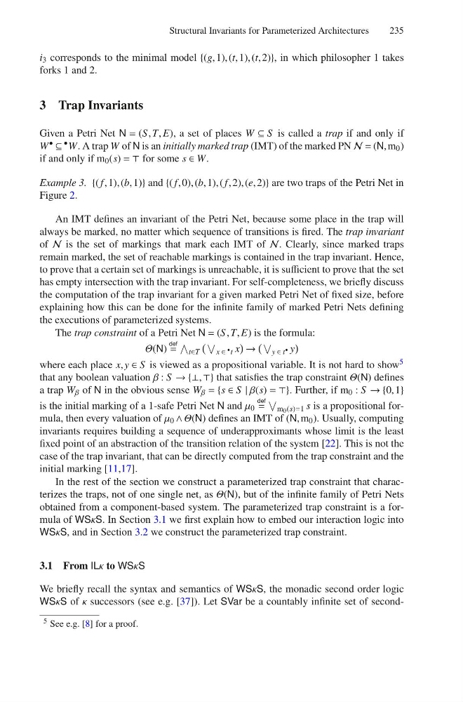
The trap constraint of a Petri Net N = (S , T, E) is the formula:
Θ(N)
def
=
t∈T
x ∈
• t x
→
y ∈ t
• y
where each place x, y ∈ S is viewed as a propositional variable. It is not hard to show 5
that any boolean valuation β : S → {⊥, } that satisfies the trap constraint Θ(N) defines
a trap W β of N in the obvious sense W β = {s ∈ S | β(s) = }. Further, if m 0 : S → {0, 1}
is the initial marking of a 1-safe Petri Net N and μ 0
def
=
m 0 (s)=1 s is a propositional formula, then every valuation of μ 0 ∧ Θ(N) defines an IMT of (N, m 0 ). Usually, computing
invariants requires building a sequence of underapproximants whose limit is the least
fixed point of an abstraction of the transition relation of the system [22]. This is not the
case of the trap invariant, that can be directly computed from the trap constraint and the
initial marking [11,17].
In the rest of the section we construct a parameterized trap constraint that characterizes the traps, not of one single net, as Θ(N), but of the infinite family of Petri Nets
obtained from a component-based system. The parameterized trap constraint is a formula of WSκS. In Section 3.1 we first explain how to embed our interaction logic into
WSκS, and in Section 3.2 we construct the parameterized trap constraint.
3.1 From ILκ to WSκS
We briefly recall the syntax and semantics of WSκS, the monadic second order logic
WSκS of κ successors (see e.g. [37]). Let SVar be a countably infinite set of second5 See e.g. [8] for a proof.
235
i 3 corresponds to the minimal model {(g, 1), (t, 1), (t, 2)}, in which philosopher 1 takes
forks 1 and 2.
3 Trap Invariants
Given a Petri Net N = (S , T, E), a set of places W ⊆ S is called a trap if and only if
W • ⊆ • W. A trap W of N is an initially marked trap (IMT) of the marked PN N = (N, m 0 )
if and only if m 0 (s) = for some s ∈ W.
Example 3. {( f, 1), (b, 1)} and {( f, 0), (b, 1), ( f, 2), (e, 2)} are two traps of the Petri Net in
Figure 2.
An IMT defines an invariant of the Petri Net, because some place in the trap will
always be marked, no matter which sequence of transitions is fired. The trap invariant
of N is the set of markings that mark each IMT of N. Clearly, since marked traps
remain marked, the set of reachable markings is contained in the trap invariant. Hence,
to prove that a certain set of markings is unreachable, it is sufficient to prove that the set
has empty intersection with the trap invariant. For self-completeness, we briefly discuss
the computation of the trap invariant for a given marked Petri Net of fixed size, before
explaining how this can be done for the infinite family of marked Petri Nets defining
the executions of parameterized systems.
The trap constraint of a Petri Net N = (S , T, E) is the formula:
Θ(N)
def
=
t∈T
x ∈
• t x
→
y ∈ t
• y
where each place x, y ∈ S is viewed as a propositional variable. It is not hard to show 5
that any boolean valuation β : S → {⊥, } that satisfies the trap constraint Θ(N) defines
a trap W β of N in the obvious sense W β = {s ∈ S | β(s) = }. Further, if m 0 : S → {0, 1}
is the initial marking of a 1-safe Petri Net N and μ 0
def
=
m 0 (s)=1 s is a propositional formula, then every valuation of μ 0 ∧ Θ(N) defines an IMT of (N, m 0 ). Usually, computing
invariants requires building a sequence of underapproximants whose limit is the least
fixed point of an abstraction of the transition relation of the system [22]. This is not the
case of the trap invariant, that can be directly computed from the trap constraint and the
initial marking [11,17].
In the rest of the section we construct a parameterized trap constraint that characterizes the traps, not of one single net, as Θ(N), but of the infinite family of Petri Nets
obtained from a component-based system. The parameterized trap constraint is a formula of WSκS. In Section 3.1 we first explain how to embed our interaction logic into
WSκS, and in Section 3.2 we construct the parameterized trap constraint.
3.1 From ILκ to WSκS
We briefly recall the syntax and semantics of WSκS, the monadic second order logic
WSκS of κ successors (see e.g. [37]). Let SVar be a countably infinite set of second5 See e.g. [8] for a proof.