

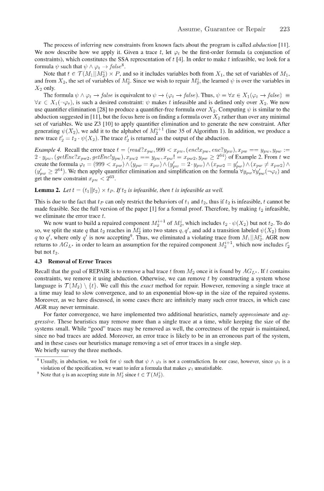
The process of inferring new constraints from known facts about the program is called abduction [11].
We now describe how we apply it. Given a trace t, let ϕ t be the first-order formula (a conjunction of
constraints), which constitutes the SSA representation of t [4]. In order to make t infeasible, we look for a
formula ψ such that ψ ∧ ϕ t → false
8 .
Note that t ∈ T (M 1 ||M
i
2 ) × P , and so it includes variables both from X 1 , the set of variables of M 1 ,
and from X 2 , the set of variables of M
i
2 . Since we wish to repair M
i
2 , the learned ψ is over the variables in
X 2 only.
The formula ψ ∧ ϕ t → false is equivalent to ψ → (ϕ t → false). Thus, ψ = ∀x ∈ X 1 (ϕ t → false) ≡
∀x ∈ X 1 (¬ϕ t ), is such a desired constraint: ψ makes t infeasible and is defined only over X 2 . We now
use quantifier elimination [28] to produce a quantifier-free formula over X 2 . Computing ψ is similar to the
abduction suggested in [11], but the focus here is on finding a formula over X 2 rather than over any minimal
set of variables. We use Z3 [10] to apply quantifier elimination and to generate the new constraint. After
generating ψ(X 2 ), we add it to the alphabet of M
i+1
2
(line 35 of Algorithm 1). In addition, we produce a
new trace t
2 = t 2 · ψ(X 2 ). The trace t
2 is returned as the output of the abduction.
Example 4. Recall the error trace t = read ?x pw , 999 < x pw , (enc!x pw , enc?y pw ), x pw == y pw , y pw :=
2 · y pw , (getEnc?x pw2 , getEnc!y pw ), x pw2 == y pw , x pw ! = x pw2 , y pw ≥ 2
64 of Example 2. From t we
create the formula ϕ t = (999 < x pw ) ∧ (y pw = x pw ) ∧ (y
pw = 2 · y pw ) ∧ (x pw2 = y
pw ) ∧ (x pw = x pw2 ) ∧
(y
pw ≥ 2
64 ). We then apply quantifier elimination and simplification on the formula ∀y pw ∀y
pw (¬ϕ t ) and
get the new constraint x pw < 2
63 .
Lemma 2. Let t = (t 1 ||t 2 ) × t P . If t 2 is infeasible, then t is infeasible as well.
This is due to the fact that t P can only restrict the behaviors of t 1 and t 2 , thus if t 2 is infeasible, t cannot be
made feasible. See the full version of the paper [1] for a formal proof. Therefore, by making t 2 infeasible,
we eliminate the error trace t.
We now want to build a repaired component M
i+1
2
of M
i
2 , which includes t 2 · ψ(X 2 ) but not t 2 . To do
so, we split the state q that t 2 reaches in M
i
2 into two states q, q
, and add a transition labeled ψ(X 2 ) from
q to q
, where only q
is now accepting
9 . Thus, we eliminated a violating trace from M 1 ||M
i
2 . AGR now
returns to AG L ∗ in order to learn an assumption for the repaired component M
i+1
2
, which now includes t
2
but not t 2 .
4.3 Removal of Error Traces
Recall that the goal of REPAIR is to remove a bad trace t from M 2 once it is found by AG L ∗ . If t contains
constraints, we remove it using abduction. Otherwise, we can remove t by constructing a system whose
language is T (M 2 ) \ {t}. We call this the exact method for repair. However, removing a single trace at
a time may lead to slow convergence, and to an exponential blow-up in the size of the repaired systems.
Moreover, as we have discussed, in some cases there are infinitely many such error traces, in which case
AGR may never terminate.
For faster convergence, we have implemented two additional heuristics, namely approximate and aggressive. These heuristics may remove more than a single trace at a time, while keeping the size of the
systems small. While “good” traces may be removed as well, the correctness of the repair is maintained,
since no bad traces are added. Moreover, an error trace is likely to be in an erroneous part of the system,
and in these cases our heuristics manage removing a set of error traces in a single step.
We briefly survey the three methods.
8 Usually, in abduction, we look for ψ such that ψ ∧ ϕt is not a contradiction. In our case, however, since ϕt is a
violation of the specification, we want to infer a formula that makes ϕt unsatisfiable.
9 Note that q is an accepting state in M
i
2 since t ∈ T (M
i
2 ).
Assume, Guarantee or Repair
223
We now describe how we apply it. Given a trace t, let ϕ t be the first-order formula (a conjunction of
constraints), which constitutes the SSA representation of t [4]. In order to make t infeasible, we look for a
formula ψ such that ψ ∧ ϕ t → false
8 .
Note that t ∈ T (M 1 ||M
i
2 ) × P , and so it includes variables both from X 1 , the set of variables of M 1 ,
and from X 2 , the set of variables of M
i
2 . Since we wish to repair M
i
2 , the learned ψ is over the variables in
X 2 only.
The formula ψ ∧ ϕ t → false is equivalent to ψ → (ϕ t → false). Thus, ψ = ∀x ∈ X 1 (ϕ t → false) ≡
∀x ∈ X 1 (¬ϕ t ), is such a desired constraint: ψ makes t infeasible and is defined only over X 2 . We now
use quantifier elimination [28] to produce a quantifier-free formula over X 2 . Computing ψ is similar to the
abduction suggested in [11], but the focus here is on finding a formula over X 2 rather than over any minimal
set of variables. We use Z3 [10] to apply quantifier elimination and to generate the new constraint. After
generating ψ(X 2 ), we add it to the alphabet of M
i+1
2
(line 35 of Algorithm 1). In addition, we produce a
new trace t
2 = t 2 · ψ(X 2 ). The trace t
2 is returned as the output of the abduction.
Example 4. Recall the error trace t = read ?x pw , 999 < x pw , (enc!x pw , enc?y pw ), x pw == y pw , y pw :=
2 · y pw , (getEnc?x pw2 , getEnc!y pw ), x pw2 == y pw , x pw ! = x pw2 , y pw ≥ 2
64 of Example 2. From t we
create the formula ϕ t = (999 < x pw ) ∧ (y pw = x pw ) ∧ (y
pw = 2 · y pw ) ∧ (x pw2 = y
pw ) ∧ (x pw = x pw2 ) ∧
(y
pw ≥ 2
64 ). We then apply quantifier elimination and simplification on the formula ∀y pw ∀y
pw (¬ϕ t ) and
get the new constraint x pw < 2
63 .
Lemma 2. Let t = (t 1 ||t 2 ) × t P . If t 2 is infeasible, then t is infeasible as well.
This is due to the fact that t P can only restrict the behaviors of t 1 and t 2 , thus if t 2 is infeasible, t cannot be
made feasible. See the full version of the paper [1] for a formal proof. Therefore, by making t 2 infeasible,
we eliminate the error trace t.
We now want to build a repaired component M
i+1
2
of M
i
2 , which includes t 2 · ψ(X 2 ) but not t 2 . To do
so, we split the state q that t 2 reaches in M
i
2 into two states q, q
, and add a transition labeled ψ(X 2 ) from
q to q
, where only q
is now accepting
9 . Thus, we eliminated a violating trace from M 1 ||M
i
2 . AGR now
returns to AG L ∗ in order to learn an assumption for the repaired component M
i+1
2
, which now includes t
2
but not t 2 .
4.3 Removal of Error Traces
Recall that the goal of REPAIR is to remove a bad trace t from M 2 once it is found by AG L ∗ . If t contains
constraints, we remove it using abduction. Otherwise, we can remove t by constructing a system whose
language is T (M 2 ) \ {t}. We call this the exact method for repair. However, removing a single trace at
a time may lead to slow convergence, and to an exponential blow-up in the size of the repaired systems.
Moreover, as we have discussed, in some cases there are infinitely many such error traces, in which case
AGR may never terminate.
For faster convergence, we have implemented two additional heuristics, namely approximate and aggressive. These heuristics may remove more than a single trace at a time, while keeping the size of the
systems small. While “good” traces may be removed as well, the correctness of the repair is maintained,
since no bad traces are added. Moreover, an error trace is likely to be in an erroneous part of the system,
and in these cases our heuristics manage removing a set of error traces in a single step.
We briefly survey the three methods.
8 Usually, in abduction, we look for ψ such that ψ ∧ ϕt is not a contradiction. In our case, however, since ϕt is a
violation of the specification, we want to infer a formula that makes ϕt unsatisfiable.
9 Note that q is an accepting state in M
i
2 since t ∈ T (M
i
2 ).
Assume, Guarantee or Repair
223