

Relational Differential Dynamic Logic
197
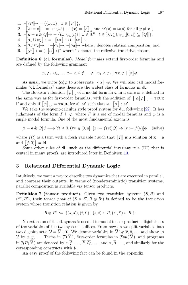
1. −
?P
→ = {(ω, ω) | ω ∈
P
},
2. −
x := e
→ = {(ω, ω
) | ω
(x) =
e
ω
and ω
(y) = ω(y) for all y = x},
3. −
˙
x = e & Q
→ = {(ω, ψ ω (t)) | ω ∈ R
V
, t ∈ [0, T ω ), ψ ω ([0, t]) ⊆
Q
},
4. −
α 1 ∪ α 2
→ = −
α 1
→ ∪ −
α 2
→,
5. −
α 1 ; α 2
→ = −
α 1
→; −
α 2
→ where ; denotes relation composition, and
6. −
α
∗
→ = (−
α
→)
∗ where
∗ denotes the reflexive transitive closure.
Definition 6 (dL formulas). Modal formulas extend first-order formulas and
are defined by the following grammar:
ϕ, ϕ 1 , ϕ 2 , . . . ::= e ≤ f | ¬ϕ | ϕ 1 ∧ ϕ 2 | ∀x. ϕ |
α
ϕ.
As usual, we write αϕ to abbreviate ¬
α
¬ϕ. We will also call modal formulas “dL formulas” since these are the widest class of formulas in dL.
The Boolean valuation
ϕ
ω
of a modal formula ϕ in a state ω is defined in
the same way as for first-order formulas, with the addition of
α
ϕ
ω
= true
if and only if
ϕ
ω = true for all ω
such that ω −
α
→ ω
.
We take the sequent-calculus style proof system for dL, following [22]. It has
judgments of the form Γ ϕ, where Γ is a set of modal formulas and ϕ is a
single modal formula. One of the most fundamental axiom is
˙
x = e & Q
φ ⇐⇒ ∀t ≥ 0. (∀v ∈ [0, u]. [x := f (v)]Q) ⇒ [x := f (u)]φ (solve)
where f (t) is a term with a fresh variable t such that
f
is a solution of ˙
x = e
and
f (0)
= id.
Some other rules of dL, such as the differential invariant rule (DI) that is
central in many proofs, are introduced later in Definition 13.
3 Relational Differential Dynamic Logic
Intuitively, we want a way to describe two dynamics that are executed in parallel,
and compare their outputs. In terms of (nondeterministic) transition systems,
parallel composition is available via tensor products.
Definition 7 (tensor product). Given two transition systems (S, R) and
(S
, R
), their tensor product (S × S
, R ⊗ R
) is defined to be the transition
system whose transition relation is given by
R ⊗ R
:= {(s, s
), (t, t
) | (s, t) ∈ R, (s
, t
) ∈ R
}.
No extension of the dL syntax is needed to model tensor products: disjointness
of the variables of the two systems suffices. From now on we split variables into
two disjoint sets: V = V V V. We denote variables in V by x, y, . . . and those in
V by x, y, . . . . Terms in T ( V ), first-order formulas in Fml ( V ), and programs
in HP( V ) are denoted by e, f, . . . , P , Q, . . . , and α, β, . . . , and similarly for the
corresponding constructs with V.
An easy proof of the following fact can be found in the appendix.
197
1. −
?P
→ = {(ω, ω) | ω ∈
P
},
2. −
x := e
→ = {(ω, ω
) | ω
(x) =
e
ω
and ω
(y) = ω(y) for all y = x},
3. −
˙
x = e & Q
→ = {(ω, ψ ω (t)) | ω ∈ R
V
, t ∈ [0, T ω ), ψ ω ([0, t]) ⊆
Q
},
4. −
α 1 ∪ α 2
→ = −
α 1
→ ∪ −
α 2
→,
5. −
α 1 ; α 2
→ = −
α 1
→; −
α 2
→ where ; denotes relation composition, and
6. −
α
∗
→ = (−
α
→)
∗ where
∗ denotes the reflexive transitive closure.
Definition 6 (dL formulas). Modal formulas extend first-order formulas and
are defined by the following grammar:
ϕ, ϕ 1 , ϕ 2 , . . . ::= e ≤ f | ¬ϕ | ϕ 1 ∧ ϕ 2 | ∀x. ϕ |
α
ϕ.
As usual, we write αϕ to abbreviate ¬
α
¬ϕ. We will also call modal formulas “dL formulas” since these are the widest class of formulas in dL.
The Boolean valuation
ϕ
ω
of a modal formula ϕ in a state ω is defined in
the same way as for first-order formulas, with the addition of
α
ϕ
ω
= true
if and only if
ϕ
ω = true for all ω
such that ω −
α
→ ω
.
We take the sequent-calculus style proof system for dL, following [22]. It has
judgments of the form Γ ϕ, where Γ is a set of modal formulas and ϕ is a
single modal formula. One of the most fundamental axiom is
˙
x = e & Q
φ ⇐⇒ ∀t ≥ 0. (∀v ∈ [0, u]. [x := f (v)]Q) ⇒ [x := f (u)]φ (solve)
where f (t) is a term with a fresh variable t such that
f
is a solution of ˙
x = e
and
f (0)
= id.
Some other rules of dL, such as the differential invariant rule (DI) that is
central in many proofs, are introduced later in Definition 13.
3 Relational Differential Dynamic Logic
Intuitively, we want a way to describe two dynamics that are executed in parallel,
and compare their outputs. In terms of (nondeterministic) transition systems,
parallel composition is available via tensor products.
Definition 7 (tensor product). Given two transition systems (S, R) and
(S
, R
), their tensor product (S × S
, R ⊗ R
) is defined to be the transition
system whose transition relation is given by
R ⊗ R
:= {(s, s
), (t, t
) | (s, t) ∈ R, (s
, t
) ∈ R
}.
No extension of the dL syntax is needed to model tensor products: disjointness
of the variables of the two systems suffices. From now on we split variables into
two disjoint sets: V = V V V. We denote variables in V by x, y, . . . and those in
V by x, y, . . . . Terms in T ( V ), first-order formulas in Fml ( V ), and programs
in HP( V ) are denoted by e, f, . . . , P , Q, . . . , and α, β, . . . , and similarly for the
corresponding constructs with V.
An easy proof of the following fact can be found in the appendix.