

162
A. Cimatti et al.
• (discrete transition) if α = τ then there is a tuple (v i , R i , Ξ i , Φ i , v i+1 ) ∈
T A such that: ν i |= inv
cl
A (v i ) ∧ Ξ i ; λ i |= Φ i ; ν i+1 = ν i [R i → 0]; ν i+1 |=
inv
cl
A (v i+1 ); λ i+1 (l A ) = v i+1 , and λ i+1 |= inv
loc
A (v i+1 ).
Definition 7 (Product of TASVs) Given two TASVs A and B, their product
is the TASV A ⊗ B defined as follows:
– V A⊗B = V A × V B and v
0
A⊗B = (v
0
A , v
0
B );
– l A⊗B = (l A , l B );
– C A⊗B = C A ∪ C B ;
– inv
cl
A⊗B (v, u) = inv
cl
A (v) ∧ inv
cl
B (u), for all (v, u) ∈ V A⊗B ;
– inv
loc
A⊗B (v, u) = inv
loc
A (v) ∧ inv
loc
B (u), for all (v, u) ∈ V A⊗B ;
– the transition relation is defined as follows:
T A⊗B ={((v, u), R, Ξ, Φ, (v
, u)) | (v, R, Ξ, Φ, v
) ∈ T A } ∪
{((v, u), R, Ξ, Φ, (v, u
)) | (u, R, Ξ, Φ, u
) ∈ T B }
It is worth noting that each TASV corresponds to a timed automaton defined
in the standard way [1], and viceversa. We define now the TASV corresponding
to a local requirement.
Definition 8 (TASV for a Local Requirement) Let C = P
C
1 , . . . , P
C
n be
a local requirement. We define the corresponding TASV A = {V A , v
0
A , l A , C A ,
inv
cl
A , inv
loc
A , T A } as follows:
– for each phase P
C
i of local requirement C, v
i
A is the corresponding location
in V A ; P
C
0 corresponds to v
0
A and C A = {c A };
– for each phase P
C
i (but the last) of C, inv
cl
A (v
i
A ) := c A ≤ u P C
i+1
;
– (discrete transition) for each phase P
C
i (but the last) of C, it holds that
(v
i
A , {c A }, Ξ
C
i , Φ P C
i+1
∧ Ψ P C
i+1
, v
i+1
A ) ∈ T A , where Ξ
C
i := l P C
i+1
≤ c A ≤ u P C
i+1
.
– (state deps) for each phase P
C
i of C, it holds that inv
loc
A (v
i
A ) := Ψ P C
i
;
where Φ P := φ P [(d, j) → (l d = v j )], for each phase P (the same holds for Ψ );
A
off
inv:
c A ≤ 6
on
3 ≤ cA ≤ 6
cA := 0
B
inv:
c B ≤ 4
inv:
ψon
2 ≤ cB ≤ 4
cB := 0
ψon
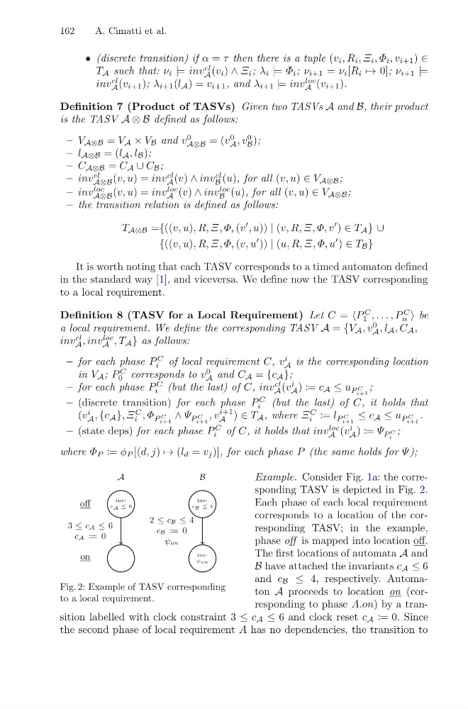
Fig. 2: Example of TASV corresponding
to a local requirement.
Example. Consider Fig. 1a: the corresponding TASV is depicted in Fig. 2.
Each phase of each local requirement
corresponds to a location of the corresponding TASV; in the example,
phase off is mapped into location off.
The first locations of automata A and
B have attached the invariants c A ≤ 6
and c B ≤ 4, respectively. Automaton A proceeds to location on (corresponding to phase A.on) by a transition labelled with clock constraint 3 ≤ c A ≤ 6 and clock reset c A := 0. Since
the second phase of local requirement A has no dependencies, the transition to
A. Cimatti et al.
• (discrete transition) if α = τ then there is a tuple (v i , R i , Ξ i , Φ i , v i+1 ) ∈
T A such that: ν i |= inv
cl
A (v i ) ∧ Ξ i ; λ i |= Φ i ; ν i+1 = ν i [R i → 0]; ν i+1 |=
inv
cl
A (v i+1 ); λ i+1 (l A ) = v i+1 , and λ i+1 |= inv
loc
A (v i+1 ).
Definition 7 (Product of TASVs) Given two TASVs A and B, their product
is the TASV A ⊗ B defined as follows:
– V A⊗B = V A × V B and v
0
A⊗B = (v
0
A , v
0
B );
– l A⊗B = (l A , l B );
– C A⊗B = C A ∪ C B ;
– inv
cl
A⊗B (v, u) = inv
cl
A (v) ∧ inv
cl
B (u), for all (v, u) ∈ V A⊗B ;
– inv
loc
A⊗B (v, u) = inv
loc
A (v) ∧ inv
loc
B (u), for all (v, u) ∈ V A⊗B ;
– the transition relation is defined as follows:
T A⊗B ={((v, u), R, Ξ, Φ, (v
, u)) | (v, R, Ξ, Φ, v
) ∈ T A } ∪
{((v, u), R, Ξ, Φ, (v, u
)) | (u, R, Ξ, Φ, u
) ∈ T B }
It is worth noting that each TASV corresponds to a timed automaton defined
in the standard way [1], and viceversa. We define now the TASV corresponding
to a local requirement.
Definition 8 (TASV for a Local Requirement) Let C = P
C
1 , . . . , P
C
n be
a local requirement. We define the corresponding TASV A = {V A , v
0
A , l A , C A ,
inv
cl
A , inv
loc
A , T A } as follows:
– for each phase P
C
i of local requirement C, v
i
A is the corresponding location
in V A ; P
C
0 corresponds to v
0
A and C A = {c A };
– for each phase P
C
i (but the last) of C, inv
cl
A (v
i
A ) := c A ≤ u P C
i+1
;
– (discrete transition) for each phase P
C
i (but the last) of C, it holds that
(v
i
A , {c A }, Ξ
C
i , Φ P C
i+1
∧ Ψ P C
i+1
, v
i+1
A ) ∈ T A , where Ξ
C
i := l P C
i+1
≤ c A ≤ u P C
i+1
.
– (state deps) for each phase P
C
i of C, it holds that inv
loc
A (v
i
A ) := Ψ P C
i
;
where Φ P := φ P [(d, j) → (l d = v j )], for each phase P (the same holds for Ψ );
A
off
inv:
c A ≤ 6
on
3 ≤ cA ≤ 6
cA := 0
B
inv:
c B ≤ 4
inv:
ψon
2 ≤ cB ≤ 4
cB := 0
ψon
Fig. 2: Example of TASV corresponding
to a local requirement.
Example. Consider Fig. 1a: the corresponding TASV is depicted in Fig. 2.
Each phase of each local requirement
corresponds to a location of the corresponding TASV; in the example,
phase off is mapped into location off.
The first locations of automata A and
B have attached the invariants c A ≤ 6
and c B ≤ 4, respectively. Automaton A proceeds to location on (corresponding to phase A.on) by a transition labelled with clock constraint 3 ≤ c A ≤ 6 and clock reset c A := 0. Since
the second phase of local requirement A has no dependencies, the transition to