

A Study of Symmetry Breaking Predicates and Model Counting
123
fact SymmetryBreaking { // pre-order
BT.root in first[]
all n: BT.root.*(left + right) {
some n.left implies n.left in next[n]
no n.left implies n.right in next[n]
some n.right and some n.left implies
n.right in next[max[n.left.*(left + right)]] }}
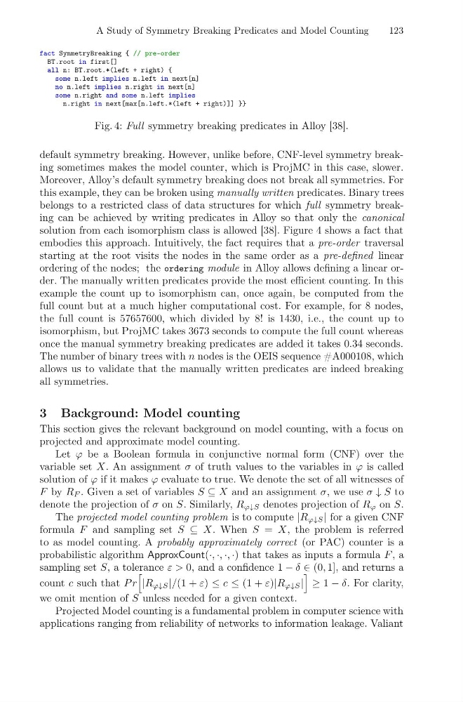
Fig. 4: Full symmetry breaking predicates in Alloy [38].
default symmetry breaking. However, unlike before, CNF-level symmetry breaking sometimes makes the model counter, which is ProjMC in this case, slower.
Moreover, Alloy’s default symmetry breaking does not break all symmetries. For
this example, they can be broken using manually written predicates. Binary trees
belongs to a restricted class of data structures for which full symmetry breaking can be achieved by writing predicates in Alloy so that only the canonical
solution from each isomorphism class is allowed [38]. Figure 4 shows a fact that
embodies this approach. Intuitively, the fact requires that a pre-order traversal
starting at the root visits the nodes in the same order as a pre-defined linear
ordering of the nodes; the ordering module in Alloy allows defining a linear order. The manually written predicates provide the most efficient counting. In this
example the count up to isomorphism can, once again, be computed from the
full count but at a much higher computational cost. For example, for 8 nodes,
the full count is 57657600, which divided by 8! is 1430, i.e., the count up to
isomorphism, but ProjMC takes 3673 seconds to compute the full count whereas
once the manual symmetry breaking predicates are added it takes 0.34 seconds.
The number of binary trees with n nodes is the OEIS sequence #A000108, which
allows us to validate that the manually written predicates are indeed breaking
all symmetries.
3 Background: Model counting
This section gives the relevant background on model counting, with a focus on
projected and approximate model counting.
Let ϕ be a Boolean formula in conjunctive normal form (CNF) over the
variable set X. An assignment σ of truth values to the variables in ϕ is called
solution of ϕ if it makes ϕ evaluate to true. We denote the set of all witnesses of
F by R F . Given a set of variables S ⊆ X and an assignment σ, we use σ ↓ S to
denote the projection of σ on S. Similarly, R ϕ↓S denotes projection of R ϕ on S.
The projected model counting problem is to compute |R ϕ↓S | for a given CNF
formula F and sampling set S ⊆ X. When S = X, the problem is referred
to as model counting. A probably approximately correct (or PAC) counter is a
probabilistic algorithm ApproxCount(·, ·, ·, ·) that takes as inputs a formula F , a
sampling set S, a tolerance ε > 0, and a confidence 1 − δ ∈ (0, 1], and returns a
count c such that P r
|R ϕ↓S |/(1 + ε) ≤ c ≤ (1 + ε)|R ϕ↓S |
≥ 1 − δ. For clarity,
we omit mention of S unless needed for a given context.
Projected Model counting is a fundamental problem in computer science with
applications ranging from reliability of networks to information leakage. Valiant
123
fact SymmetryBreaking { // pre-order
BT.root in first[]
all n: BT.root.*(left + right) {
some n.left implies n.left in next[n]
no n.left implies n.right in next[n]
some n.right and some n.left implies
n.right in next[max[n.left.*(left + right)]] }}
Fig. 4: Full symmetry breaking predicates in Alloy [38].
default symmetry breaking. However, unlike before, CNF-level symmetry breaking sometimes makes the model counter, which is ProjMC in this case, slower.
Moreover, Alloy’s default symmetry breaking does not break all symmetries. For
this example, they can be broken using manually written predicates. Binary trees
belongs to a restricted class of data structures for which full symmetry breaking can be achieved by writing predicates in Alloy so that only the canonical
solution from each isomorphism class is allowed [38]. Figure 4 shows a fact that
embodies this approach. Intuitively, the fact requires that a pre-order traversal
starting at the root visits the nodes in the same order as a pre-defined linear
ordering of the nodes; the ordering module in Alloy allows defining a linear order. The manually written predicates provide the most efficient counting. In this
example the count up to isomorphism can, once again, be computed from the
full count but at a much higher computational cost. For example, for 8 nodes,
the full count is 57657600, which divided by 8! is 1430, i.e., the count up to
isomorphism, but ProjMC takes 3673 seconds to compute the full count whereas
once the manual symmetry breaking predicates are added it takes 0.34 seconds.
The number of binary trees with n nodes is the OEIS sequence #A000108, which
allows us to validate that the manually written predicates are indeed breaking
all symmetries.
3 Background: Model counting
This section gives the relevant background on model counting, with a focus on
projected and approximate model counting.
Let ϕ be a Boolean formula in conjunctive normal form (CNF) over the
variable set X. An assignment σ of truth values to the variables in ϕ is called
solution of ϕ if it makes ϕ evaluate to true. We denote the set of all witnesses of
F by R F . Given a set of variables S ⊆ X and an assignment σ, we use σ ↓ S to
denote the projection of σ on S. Similarly, R ϕ↓S denotes projection of R ϕ on S.
The projected model counting problem is to compute |R ϕ↓S | for a given CNF
formula F and sampling set S ⊆ X. When S = X, the problem is referred
to as model counting. A probably approximately correct (or PAC) counter is a
probabilistic algorithm ApproxCount(·, ·, ·, ·) that takes as inputs a formula F , a
sampling set S, a tolerance ε > 0, and a confidence 1 − δ ∈ (0, 1], and returns a
count c such that P r
|R ϕ↓S |/(1 + ε) ≤ c ≤ (1 + ε)|R ϕ↓S |
≥ 1 − δ. For clarity,
we omit mention of S unless needed for a given context.
Projected Model counting is a fundamental problem in computer science with
applications ranging from reliability of networks to information leakage. Valiant