

Automated and Sound Synthesis of Lyapunov Functions with SMT Solvers
111
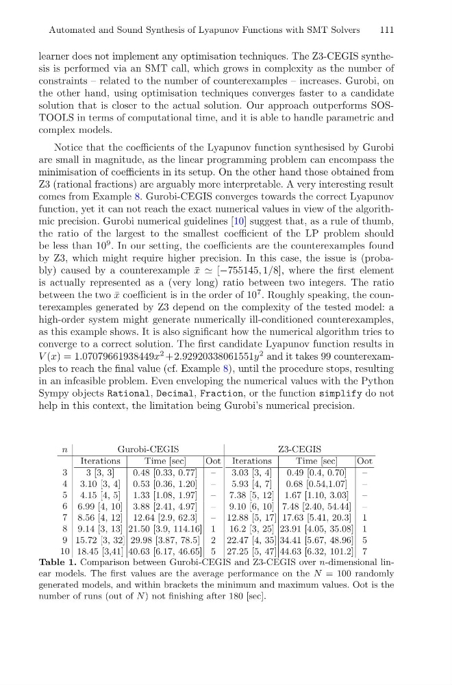
learner does not implement any optimisation techniques. The Z3-CEGIS synthesis is performed via an SMT call, which grows in complexity as the number of
constraints – related to the number of counterexamples – increases. Gurobi, on
the other hand, using optimisation techniques converges faster to a candidate
solution that is closer to the actual solution. Our approach outperforms SOSTOOLS in terms of computational time, and it is able to handle parametric and
complex models.
Notice that the coefficients of the Lyapunov function synthesised by Gurobi
are small in magnitude, as the linear programming problem can encompass the
minimisation of coefficients in its setup. On the other hand those obtained from
Z3 (rational fractions) are arguably more interpretable. A very interesting result
comes from Example 8. Gurobi-CEGIS converges towards the correct Lyapunov
function, yet it can not reach the exact numerical values in view of the algorithmic precision. Gurobi numerical guidelines [10] suggest that, as a rule of thumb,
the ratio of the largest to the smallest coefficient of the LP problem should
be less than 10
9 . In our setting, the coefficients are the counterexamples found
by Z3, which might require higher precision. In this case, the issue is (probably) caused by a counterexample ¯
x [−755145, 1/8], where the first element
is actually represented as a (very long) ratio between two integers. The ratio
between the two ¯
x coefficient is in the order of 10
7 . Roughly speaking, the counterexamples generated by Z3 depend on the complexity of the tested model: a
high-order system might generate numerically ill-conditioned counterexamples,
as this example shows. It is also significant how the numerical algorithm tries to
converge to a correct solution. The first candidate Lyapunov function results in
V (x) = 1.07079661938449x
2 +2.92920338061551y
2 and it takes 99 counterexamples to reach the final value (cf. Example 8), until the procedure stops, resulting
in an infeasible problem. Even enveloping the numerical values with the Python
Sympy objects Rational, Decimal, Fraction, or the function simplify do not
help in this context, the limitation being Gurobi’s numerical precision.
n
Gurobi-CEGIS
Z3-CEGIS
3
4
5
6
7
8
9
10
Iterations
Time [sec]
Oot
3 [3, 3]
0.48 [0.33, 0.77] –
3.10 [3, 4] 0.53 [0.36, 1.20] –
4.15 [4, 5] 1.33 [1.08, 1.97] –
6.99 [4, 10] 3.88 [2.41, 4.97] –
8.56 [4, 12] 12.64 [2.9, 62.3] –
9.14 [3, 13] 21.50 [3.9, 114.16] 1
15.72 [3, 32] 29.98 [3.87, 78.5] 2
18.45 [3,41] 40.63 [6.17, 46.65] 5
Iterations
Time [sec]
Oot
3.03 [3, 4]
0.49 [0.4, 0.70]
–
5.93 [4, 7]
0.68 [0.54,1.07]
–
7.38 [5, 12] 1.67 [1.10, 3.03] –
9.10 [6, 10] 7.48 [2.40, 54.44] –
12.88 [5, 17] 17.63 [5.41, 20.3] 1
16.2 [3, 25] 23.91 [4.05, 35.08] 1
22.47 [4, 35] 34.41 [5.67, 48.96] 5
27.25 [5, 47] 44.63 [6.32, 101.2] 7
Table 1. Comparison between Gurobi-CEGIS and Z3-CEGIS over n-dimensional linear models. The first values are the average performance on the N = 100 randomly
generated models, and within brackets the minimum and maximum values. Oot is the
number of runs (out of N ) not finishing after 180 [sec].
111
learner does not implement any optimisation techniques. The Z3-CEGIS synthesis is performed via an SMT call, which grows in complexity as the number of
constraints – related to the number of counterexamples – increases. Gurobi, on
the other hand, using optimisation techniques converges faster to a candidate
solution that is closer to the actual solution. Our approach outperforms SOSTOOLS in terms of computational time, and it is able to handle parametric and
complex models.
Notice that the coefficients of the Lyapunov function synthesised by Gurobi
are small in magnitude, as the linear programming problem can encompass the
minimisation of coefficients in its setup. On the other hand those obtained from
Z3 (rational fractions) are arguably more interpretable. A very interesting result
comes from Example 8. Gurobi-CEGIS converges towards the correct Lyapunov
function, yet it can not reach the exact numerical values in view of the algorithmic precision. Gurobi numerical guidelines [10] suggest that, as a rule of thumb,
the ratio of the largest to the smallest coefficient of the LP problem should
be less than 10
9 . In our setting, the coefficients are the counterexamples found
by Z3, which might require higher precision. In this case, the issue is (probably) caused by a counterexample ¯
x [−755145, 1/8], where the first element
is actually represented as a (very long) ratio between two integers. The ratio
between the two ¯
x coefficient is in the order of 10
7 . Roughly speaking, the counterexamples generated by Z3 depend on the complexity of the tested model: a
high-order system might generate numerically ill-conditioned counterexamples,
as this example shows. It is also significant how the numerical algorithm tries to
converge to a correct solution. The first candidate Lyapunov function results in
V (x) = 1.07079661938449x
2 +2.92920338061551y
2 and it takes 99 counterexamples to reach the final value (cf. Example 8), until the procedure stops, resulting
in an infeasible problem. Even enveloping the numerical values with the Python
Sympy objects Rational, Decimal, Fraction, or the function simplify do not
help in this context, the limitation being Gurobi’s numerical precision.
n
Gurobi-CEGIS
Z3-CEGIS
3
4
5
6
7
8
9
10
Iterations
Time [sec]
Oot
3 [3, 3]
0.48 [0.33, 0.77] –
3.10 [3, 4] 0.53 [0.36, 1.20] –
4.15 [4, 5] 1.33 [1.08, 1.97] –
6.99 [4, 10] 3.88 [2.41, 4.97] –
8.56 [4, 12] 12.64 [2.9, 62.3] –
9.14 [3, 13] 21.50 [3.9, 114.16] 1
15.72 [3, 32] 29.98 [3.87, 78.5] 2
18.45 [3,41] 40.63 [6.17, 46.65] 5
Iterations
Time [sec]
Oot
3.03 [3, 4]
0.49 [0.4, 0.70]
–
5.93 [4, 7]
0.68 [0.54,1.07]
–
7.38 [5, 12] 1.67 [1.10, 3.03] –
9.10 [6, 10] 7.48 [2.40, 54.44] –
12.88 [5, 17] 17.63 [5.41, 20.3] 1
16.2 [3, 25] 23.91 [4.05, 35.08] 1
22.47 [4, 35] 34.41 [5.67, 48.96] 5
27.25 [5, 47] 44.63 [6.32, 101.2] 7
Table 1. Comparison between Gurobi-CEGIS and Z3-CEGIS over n-dimensional linear models. The first values are the average performance on the N = 100 randomly
generated models, and within brackets the minimum and maximum values. Oot is the
number of runs (out of N ) not finishing after 180 [sec].