

92
T. Okudono and A. King
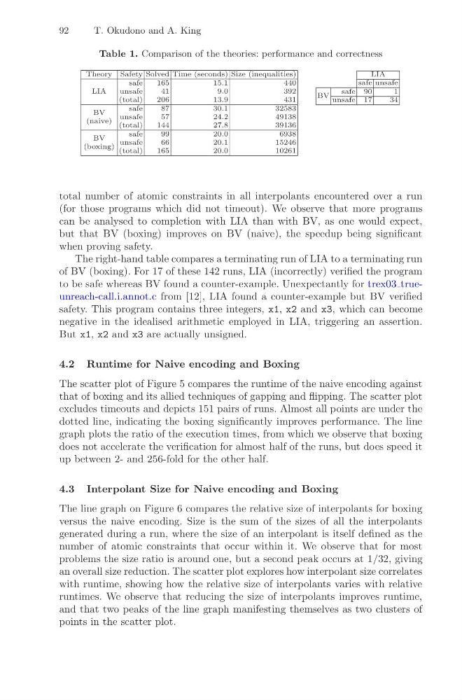
Table 1. Comparison of the theories: performance and correctness
Theory Safety Solved Time (seconds) Size (inequalities)
LIA
safe
165
15.1
440
unsafe
41
9.0
392
(total)
206
13.9
431
BV
(naive)
safe
87
30.1
32583
unsafe
57
24.2
49138
(total)
144
27.8
39136
BV
(boxing)
safe
99
20.0
6938
unsafe
66
20.1
15246
(total)
165
20.0
10261
LIA
safe unsafe
BV
safe 90
1
unsafe 17
34
total number of atomic constraints in all interpolants encountered over a run
(for those programs which did not timeout). We observe that more programs
can be analysed to completion with LIA than with BV, as one would expect,
but that BV (boxing) improves on BV (naive), the speedup being significant
when proving safety.
The right-hand table compares a terminating run of LIA to a terminating run
of BV (boxing). For 17 of these 142 runs, LIA (incorrectly) verified the program
to be safe whereas BV found a counter-example. Unexpectantly for trex03 trueunreach-call.i.annot.c from [12], LIA found a counter-example but BV verified
safety. This program contains three integers, x1, x2 and x3, which can become
negative in the idealised arithmetic employed in LIA, triggering an assertion.
But x1, x2 and x3 are actually unsigned.
4.2 Runtime for Naive encoding and Boxing
The scatter plot of Figure 5 compares the runtime of the naive encoding against
that of boxing and its allied techniques of gapping and flipping. The scatter plot
excludes timeouts and depicts 151 pairs of runs. Almost all points are under the
dotted line, indicating the boxing significantly improves performance. The line
graph plots the ratio of the execution times, from which we observe that boxing
does not accelerate the verification for almost half of the runs, but does speed it
up between 2- and 256-fold for the other half.
4.3 Interpolant Size for Naive encoding and Boxing
The line graph on Figure 6 compares the relative size of interpolants for boxing
versus the naive encoding. Size is the sum of the sizes of all the interpolants
generated during a run, where the size of an interpolant is itself defined as the
number of atomic constraints that occur within it. We observe that for most
problems the size ratio is around one, but a second peak occurs at 1/32, giving
an overall size reduction. The scatter plot explores how interpolant size correlates
with runtime, showing how the relative size of interpolants varies with relative
runtimes. We observe that reducing the size of interpolants improves runtime,
and that two peaks of the line graph manifesting themselves as two clusters of
points in the scatter plot.
T. Okudono and A. King
Table 1. Comparison of the theories: performance and correctness
Theory Safety Solved Time (seconds) Size (inequalities)
LIA
safe
165
15.1
440
unsafe
41
9.0
392
(total)
206
13.9
431
BV
(naive)
safe
87
30.1
32583
unsafe
57
24.2
49138
(total)
144
27.8
39136
BV
(boxing)
safe
99
20.0
6938
unsafe
66
20.1
15246
(total)
165
20.0
10261
LIA
safe unsafe
BV
safe 90
1
unsafe 17
34
total number of atomic constraints in all interpolants encountered over a run
(for those programs which did not timeout). We observe that more programs
can be analysed to completion with LIA than with BV, as one would expect,
but that BV (boxing) improves on BV (naive), the speedup being significant
when proving safety.
The right-hand table compares a terminating run of LIA to a terminating run
of BV (boxing). For 17 of these 142 runs, LIA (incorrectly) verified the program
to be safe whereas BV found a counter-example. Unexpectantly for trex03 trueunreach-call.i.annot.c from [12], LIA found a counter-example but BV verified
safety. This program contains three integers, x1, x2 and x3, which can become
negative in the idealised arithmetic employed in LIA, triggering an assertion.
But x1, x2 and x3 are actually unsigned.
4.2 Runtime for Naive encoding and Boxing
The scatter plot of Figure 5 compares the runtime of the naive encoding against
that of boxing and its allied techniques of gapping and flipping. The scatter plot
excludes timeouts and depicts 151 pairs of runs. Almost all points are under the
dotted line, indicating the boxing significantly improves performance. The line
graph plots the ratio of the execution times, from which we observe that boxing
does not accelerate the verification for almost half of the runs, but does speed it
up between 2- and 256-fold for the other half.
4.3 Interpolant Size for Naive encoding and Boxing
The line graph on Figure 6 compares the relative size of interpolants for boxing
versus the naive encoding. Size is the sum of the sizes of all the interpolants
generated during a run, where the size of an interpolant is itself defined as the
number of atomic constraints that occur within it. We observe that for most
problems the size ratio is around one, but a second peak occurs at 1/32, giving
an overall size reduction. The scatter plot explores how interpolant size correlates
with runtime, showing how the relative size of interpolants varies with relative
runtimes. We observe that reducing the size of interpolants improves runtime,
and that two peaks of the line graph manifesting themselves as two clusters of
points in the scatter plot.