

Modeling Species Distribution with GIS
417
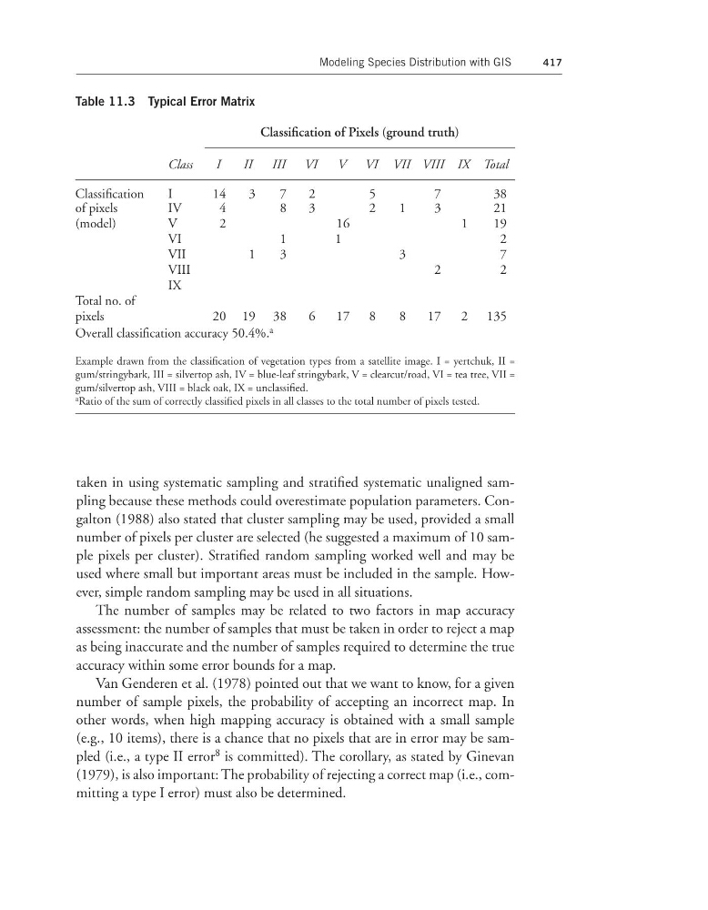
Table 11.3 Typical Error Matrix
Classification of Pixels (ground truth)
Class
I
II III VI
V VI VII VIII IX Total
Classification
I
14
3
7
2
5
7
38
of pixels
IV
4
8
3
2
1
3
21
(model)
V
2
16
1
19
VI
1
1
2
VII
1
3
3
7
VIII
2
2
IX
Total no. of
pixels
20 19 38
6
17 8
8
17
2 135
Overall classification accuracy 50.4%. a
Example drawn from the classification of vegetation types from a satellite image. I = yertchuk, II =
gum/stringybark, III = silvertop ash, IV = blue-leaf stringybark, V = clearcut/road, VI = tea tree, VII =
gum/silvertop ash, VIII = black oak, IX = unclassified.
a Ratio of the sum of correctly classified pixels in all classes to the total number of pixels tested.
taken in using systematic sampling and stratified systematic unaligned sampling because these methods could overestimate population parameters. Congalton (1988) also stated that cluster sampling may be used, provided a small
number of pixels per cluster are selected (he suggested a maximum of 10 sample pixels per cluster). Stratified random sampling worked well and may be
used where small but important areas must be included in the sample. However, simple random sampling may be used in all situations.
The number of samples may be related to two factors in map accuracy
assessment: the number of samples that must be taken in order to reject a map
as being inaccurate and the number of samples required to determine the true
accuracy within some error bounds for a map.
Van Genderen et al. (1978) pointed out that we want to know, for a given
number of sample pixels, the probability of accepting an incorrect map. In
other words, when high mapping accuracy is obtained with a small sample
(e.g., 10 items), there is a chance that no pixels that are in error may be sampled (i.e., a type II error 8 is committed). The corollary, as stated by Ginevan
(1979), is also important: The probability of rejecting a correct map (i.e., committing a type I error) must also be determined.
417
Table 11.3 Typical Error Matrix
Classification of Pixels (ground truth)
Class
I
II III VI
V VI VII VIII IX Total
Classification
I
14
3
7
2
5
7
38
of pixels
IV
4
8
3
2
1
3
21
(model)
V
2
16
1
19
VI
1
1
2
VII
1
3
3
7
VIII
2
2
IX
Total no. of
pixels
20 19 38
6
17 8
8
17
2 135
Overall classification accuracy 50.4%. a
Example drawn from the classification of vegetation types from a satellite image. I = yertchuk, II =
gum/stringybark, III = silvertop ash, IV = blue-leaf stringybark, V = clearcut/road, VI = tea tree, VII =
gum/silvertop ash, VIII = black oak, IX = unclassified.
a Ratio of the sum of correctly classified pixels in all classes to the total number of pixels tested.
taken in using systematic sampling and stratified systematic unaligned sampling because these methods could overestimate population parameters. Congalton (1988) also stated that cluster sampling may be used, provided a small
number of pixels per cluster are selected (he suggested a maximum of 10 sample pixels per cluster). Stratified random sampling worked well and may be
used where small but important areas must be included in the sample. However, simple random sampling may be used in all situations.
The number of samples may be related to two factors in map accuracy
assessment: the number of samples that must be taken in order to reject a map
as being inaccurate and the number of samples required to determine the true
accuracy within some error bounds for a map.
Van Genderen et al. (1978) pointed out that we want to know, for a given
number of sample pixels, the probability of accepting an incorrect map. In
other words, when high mapping accuracy is obtained with a small sample
(e.g., 10 items), there is a chance that no pixels that are in error may be sampled (i.e., a type II error 8 is committed). The corollary, as stated by Ginevan
(1979), is also important: The probability of rejecting a correct map (i.e., committing a type I error) must also be determined.