

410
C O R S I , D E L E E U W, A N D S K I D M O R E
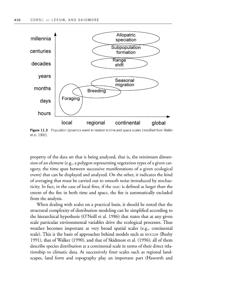
Figure 11.3 Population dynamics event in relation to time and space scales (modified from Wallin
et al. 1992).
property of the data set that is being analyzed, that is, the minimum dimension of an element (e.g., a polygon representing vegetation types of a given category, the time span between successive manifestations of a given ecological
event) that can be displayed and analyzed. On the other, it indicates the kind
of averaging that must be carried out to smooth noise introduced by stochasticity. In fact, in the case of local fires, if the MMU is defined as larger than the
extent of the fire in both time and space, the fire is automatically excluded
from the analysis.
When dealing with scales on a practical basis, it should be noted that the
structural complexity of distribution modeling can be simplified according to
the hierarchical hypothesis (O’Neill et al. 1986) that states that at any given
scale particular environmental variables drive the ecological processes. Thus
weather becomes important at very broad spatial scales (e.g., continental
scale). This is the basis of approaches behind models such as BIOCLIM (Busby
1991), that of Walker (1990), and that of Skidmore et al. (1996); all of them
describe species distribution at a continental scale in terms of their direct relationship to climatic data. At successively finer scales such as regional landscapes, land form and topography play an important part (Haworth and
C O R S I , D E L E E U W, A N D S K I D M O R E
Figure 11.3 Population dynamics event in relation to time and space scales (modified from Wallin
et al. 1992).
property of the data set that is being analyzed, that is, the minimum dimension of an element (e.g., a polygon representing vegetation types of a given category, the time span between successive manifestations of a given ecological
event) that can be displayed and analyzed. On the other, it indicates the kind
of averaging that must be carried out to smooth noise introduced by stochasticity. In fact, in the case of local fires, if the MMU is defined as larger than the
extent of the fire in both time and space, the fire is automatically excluded
from the analysis.
When dealing with scales on a practical basis, it should be noted that the
structural complexity of distribution modeling can be simplified according to
the hierarchical hypothesis (O’Neill et al. 1986) that states that at any given
scale particular environmental variables drive the ecological processes. Thus
weather becomes important at very broad spatial scales (e.g., continental
scale). This is the basis of approaches behind models such as BIOCLIM (Busby
1991), that of Walker (1990), and that of Skidmore et al. (1996); all of them
describe species distribution at a continental scale in terms of their direct relationship to climatic data. At successively finer scales such as regional landscapes, land form and topography play an important part (Haworth and