

298
G A R Y C . W H I T E
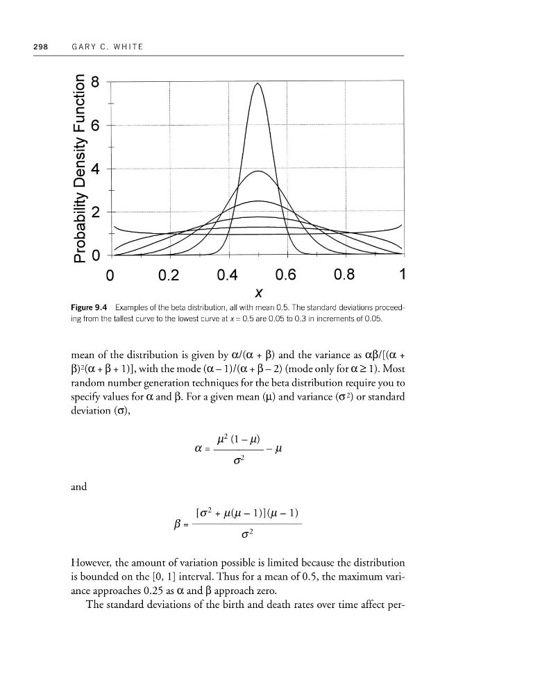
Figure 9.4 Examples of the beta distribution, all with mean 0.5. The standard deviations proceeding from the tallest curve to the lowest curve at x = 0.5 are 0.05 to 0.3 in increments of 0.05.
mean of the distribution is given by α/(α + β) and the variance as αβ/[(α +
β) 2 (α + β + 1)], with the mode (α – 1)/(α + β – 2) (mode only for α ≥ 1). Most
random number generation techniques for the beta distribution require you to
specify values for α and β. For a given mean (µ) and variance (σ 2 ) or standard
deviation (σ),
α = ᎏ
µ 2 (
σ
1
2
– µ)
ᎏ – µ
and
β =
However, the amount of variation possible is limited because the distribution
is bounded on the [0, 1] interval. Thus for a mean of 0.5, the maximum variance approaches 0.25 as α and β approach zero.
The standard deviations of the birth and death rates over time affect per[σ 2 + µ(µ – 1)](µ – 1)
ᎏᎏᎏ
σ 2
G A R Y C . W H I T E
Figure 9.4 Examples of the beta distribution, all with mean 0.5. The standard deviations proceeding from the tallest curve to the lowest curve at x = 0.5 are 0.05 to 0.3 in increments of 0.05.
mean of the distribution is given by α/(α + β) and the variance as αβ/[(α +
β) 2 (α + β + 1)], with the mode (α – 1)/(α + β – 2) (mode only for α ≥ 1). Most
random number generation techniques for the beta distribution require you to
specify values for α and β. For a given mean (µ) and variance (σ 2 ) or standard
deviation (σ),
α = ᎏ
µ 2 (
σ
1
2
– µ)
ᎏ – µ
and
β =
However, the amount of variation possible is limited because the distribution
is bounded on the [0, 1] interval. Thus for a mean of 0.5, the maximum variance approaches 0.25 as α and β approach zero.
The standard deviations of the birth and death rates over time affect per[σ 2 + µ(µ – 1)](µ – 1)
ᎏᎏᎏ
σ 2