

296
G A R Y C . W H I T E
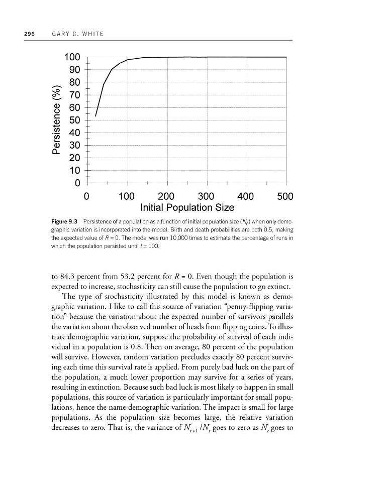
Figure 9.3 Persistence of a population as a function of initial population size (N 0 ) when only demographic variation is incorporated into the model. Birth and death probabilities are both 0.5, making
the expected value of R = 0. The model was run 10,000 times to estimate the percentage of runs in
which the population persisted until t = 100.
to 84.3 percent from 53.2 percent for R = 0. Even though the population is
expected to increase, stochasticity can still cause the population to go extinct.
The type of stochasticity illustrated by this model is known as demographic variation. I like to call this source of variation “penny-flipping variation” because the variation about the expected number of survivors parallels
the variation about the observed number of heads from flipping coins. To illustrate demographic variation, suppose the probability of survival of each individual in a population is 0.8. Then on average, 80 percent of the population
will survive. However, random variation precludes exactly 80 percent surviving each time this survival rate is applied. From purely bad luck on the part of
the population, a much lower proportion may survive for a series of years,
resulting in extinction. Because such bad luck is most likely to happen in small
populations, this source of variation is particularly important for small populations, hence the name demographic variation. The impact is small for large
populations. As the population size becomes large, the relative variation
decreases to zero. That is, the variance of N t +1 /N t goes to zero as N t goes to
G A R Y C . W H I T E
Figure 9.3 Persistence of a population as a function of initial population size (N 0 ) when only demographic variation is incorporated into the model. Birth and death probabilities are both 0.5, making
the expected value of R = 0. The model was run 10,000 times to estimate the percentage of runs in
which the population persisted until t = 100.
to 84.3 percent from 53.2 percent for R = 0. Even though the population is
expected to increase, stochasticity can still cause the population to go extinct.
The type of stochasticity illustrated by this model is known as demographic variation. I like to call this source of variation “penny-flipping variation” because the variation about the expected number of survivors parallels
the variation about the observed number of heads from flipping coins. To illustrate demographic variation, suppose the probability of survival of each individual in a population is 0.8. Then on average, 80 percent of the population
will survive. However, random variation precludes exactly 80 percent surviving each time this survival rate is applied. From purely bad luck on the part of
the population, a much lower proportion may survive for a series of years,
resulting in extinction. Because such bad luck is most likely to happen in small
populations, this source of variation is particularly important for small populations, hence the name demographic variation. The impact is small for large
populations. As the population size becomes large, the relative variation
decreases to zero. That is, the variance of N t +1 /N t goes to zero as N t goes to