

Modeling Predator–Prey Dynamics
271
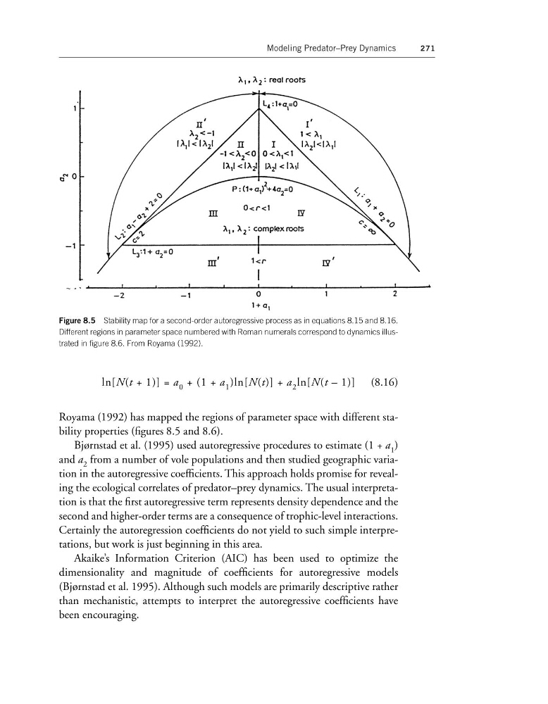
Figure 8.5 Stability map for a second-order autoregressive process as in equations 8.15 and 8.16.
Different regions in parameter space numbered with Roman numerals correspond to dynamics illustrated in figure 8.6. From Royama (1992).
ln[N(t + 1)] = a 0 + (1 + a 1 )ln[N(t)] + a 2 ln[N(t – 1)] (8.16)
Royama (1992) has mapped the regions of parameter space with different stability properties (figures 8.5 and 8.6).
Bjørnstad et al. (1995) used autoregressive procedures to estimate (1 + a 1 )
and a 2 from a number of vole populations and then studied geographic variation in the autoregressive coefficients. This approach holds promise for revealing the ecological correlates of predator–prey dynamics. The usual interpretation is that the first autoregressive term represents density dependence and the
second and higher-order terms are a consequence of trophic-level interactions.
Certainly the autoregression coefficients do not yield to such simple interpretations, but work is just beginning in this area.
Akaike’s Information Criterion (AIC) has been used to optimize the
dimensionality and magnitude of coefficients for autoregressive models
(Bjørnstad et al. 1995). Although such models are primarily descriptive rather
than mechanistic, attempts to interpret the autoregressive coefficients have
been encouraging.
271
Figure 8.5 Stability map for a second-order autoregressive process as in equations 8.15 and 8.16.
Different regions in parameter space numbered with Roman numerals correspond to dynamics illustrated in figure 8.6. From Royama (1992).
ln[N(t + 1)] = a 0 + (1 + a 1 )ln[N(t)] + a 2 ln[N(t – 1)] (8.16)
Royama (1992) has mapped the regions of parameter space with different stability properties (figures 8.5 and 8.6).
Bjørnstad et al. (1995) used autoregressive procedures to estimate (1 + a 1 )
and a 2 from a number of vole populations and then studied geographic variation in the autoregressive coefficients. This approach holds promise for revealing the ecological correlates of predator–prey dynamics. The usual interpretation is that the first autoregressive term represents density dependence and the
second and higher-order terms are a consequence of trophic-level interactions.
Certainly the autoregression coefficients do not yield to such simple interpretations, but work is just beginning in this area.
Akaike’s Information Criterion (AIC) has been used to optimize the
dimensionality and magnitude of coefficients for autoregressive models
(Bjørnstad et al. 1995). Although such models are primarily descriptive rather
than mechanistic, attempts to interpret the autoregressive coefficients have
been encouraging.