

Modeling Predator–Prey Dynamics
263
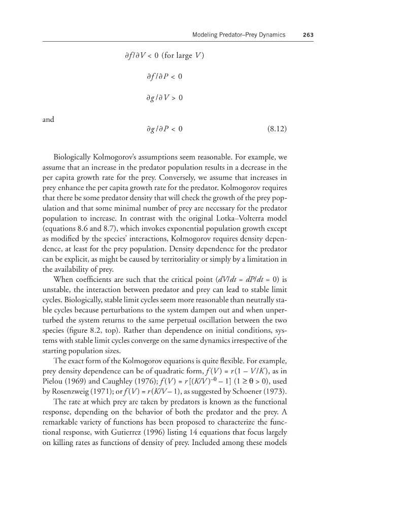
ץf /ץV < 0 (for large V )
ץf /ץP < 0
ץg /ץV > 0
and
ץg /ץP < 0
(8.12)
Biologically Kolmogorov’s assumptions seem reasonable. For example, we
assume that an increase in the predator population results in a decrease in the
per capita growth rate for the prey. Conversely, we assume that increases in
prey enhance the per capita growth rate for the predator. Kolmogorov requires
that there be some predator density that will check the growth of the prey population and that some minimal number of prey are necessary for the predator
population to increase. In contrast with the original Lotka–Volterra model
(equations 8.6 and 8.7), which invokes exponential population growth except
as modified by the species’ interactions, Kolmogorov requires density dependence, at least for the prey population. Density dependence for the predator
can be explicit, as might be caused by territoriality or simply by a limitation in
the availability of prey.
When coefficients are such that the critical point (dV/dt = dP/dt = 0) is
unstable, the interaction between predator and prey can lead to stable limit
cycles. Biologically, stable limit cycles seem more reasonable than neutrally stable cycles because perturbations to the system dampen out and when unperturbed the system returns to the same perpetual oscillation between the two
species (figure 8.2, top). Rather than dependence on initial conditions, systems with stable limit cycles converge on the same dynamics irrespective of the
starting population sizes.
The exact form of the Kolmogorov equations is quite flexible. For example,
prey density dependence can be of quadratic form, f (V ) = r (1 – V /K ), as in
Pielou (1969) and Caughley (1976); f (V ) = r [(K/V ) –θ – 1] (1 ≥ θ > 0), used
by Rosenzweig (1971); or f (V ) = r (K/V – 1), as suggested by Schoener (1973).
The rate at which prey are taken by predators is known as the functional
response, depending on the behavior of both the predator and the prey. A
remarkable variety of functions has been proposed to characterize the functional response, with Gutierrez (1996) listing 14 equations that focus largely
on killing rates as functions of density of prey. Included among these models
263
ץf /ץV < 0 (for large V )
ץf /ץP < 0
ץg /ץV > 0
and
ץg /ץP < 0
(8.12)
Biologically Kolmogorov’s assumptions seem reasonable. For example, we
assume that an increase in the predator population results in a decrease in the
per capita growth rate for the prey. Conversely, we assume that increases in
prey enhance the per capita growth rate for the predator. Kolmogorov requires
that there be some predator density that will check the growth of the prey population and that some minimal number of prey are necessary for the predator
population to increase. In contrast with the original Lotka–Volterra model
(equations 8.6 and 8.7), which invokes exponential population growth except
as modified by the species’ interactions, Kolmogorov requires density dependence, at least for the prey population. Density dependence for the predator
can be explicit, as might be caused by territoriality or simply by a limitation in
the availability of prey.
When coefficients are such that the critical point (dV/dt = dP/dt = 0) is
unstable, the interaction between predator and prey can lead to stable limit
cycles. Biologically, stable limit cycles seem more reasonable than neutrally stable cycles because perturbations to the system dampen out and when unperturbed the system returns to the same perpetual oscillation between the two
species (figure 8.2, top). Rather than dependence on initial conditions, systems with stable limit cycles converge on the same dynamics irrespective of the
starting population sizes.
The exact form of the Kolmogorov equations is quite flexible. For example,
prey density dependence can be of quadratic form, f (V ) = r (1 – V /K ), as in
Pielou (1969) and Caughley (1976); f (V ) = r [(K/V ) –θ – 1] (1 ≥ θ > 0), used
by Rosenzweig (1971); or f (V ) = r (K/V – 1), as suggested by Schoener (1973).
The rate at which prey are taken by predators is known as the functional
response, depending on the behavior of both the predator and the prey. A
remarkable variety of functions has been proposed to characterize the functional response, with Gutierrez (1996) listing 14 equations that focus largely
on killing rates as functions of density of prey. Included among these models