

256
M A R K S . B O Y C E
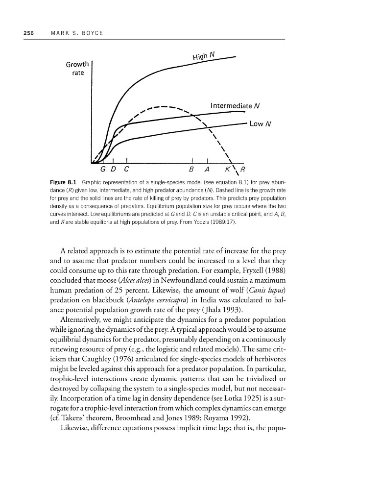
Figure 8.1 Graphic representation of a single-species model (see equation 8.1) for prey abundance (R) given low, intermediate, and high predator abundance (N). Dashed line is the growth rate
for prey and the solid lines are the rate of killing of prey by predators. This predicts prey population
density as a consequence of predators. Equilibrium population size for prey occurs where the two
curves intersect. Low equilibriums are predicted at G and D. C is an unstable critical point, and A, B,
and K are stable equilibria at high populations of prey. From Yodzis (1989:17).
A related approach is to estimate the potential rate of increase for the prey
and to assume that predator numbers could be increased to a level that they
could consume up to this rate through predation. For example, Fryxell (1988)
concluded that moose (Alces alces) in Newfoundland could sustain a maximum
human predation of 25 percent. Likewise, the amount of wolf (Canis lupus)
predation on blackbuck (Antelope cervicapra) in India was calculated to balance potential population growth rate of the prey ( Jhala 1993).
Alternatively, we might anticipate the dynamics for a predator population
while ignoring the dynamics of the prey. A typical approach would be to assume
equilibrial dynamics for the predator, presumably depending on a continuously
renewing resource of prey (e.g., the logistic and related models). The same criticism that Caughley (1976) articulated for single-species models of herbivores
might be leveled against this approach for a predator population. In particular,
trophic-level interactions create dynamic patterns that can be trivialized or
destroyed by collapsing the system to a single-species model, but not necessarily. Incorporation of a time lag in density dependence (see Lotka 1925) is a surrogate for a trophic-level interaction from which complex dynamics can emerge
(cf. Takens’ theorem, Broomhead and Jones 1989; Royama 1992).
Likewise, difference equations possess implicit time lags; that is, the popu-
M A R K S . B O Y C E
Figure 8.1 Graphic representation of a single-species model (see equation 8.1) for prey abundance (R) given low, intermediate, and high predator abundance (N). Dashed line is the growth rate
for prey and the solid lines are the rate of killing of prey by predators. This predicts prey population
density as a consequence of predators. Equilibrium population size for prey occurs where the two
curves intersect. Low equilibriums are predicted at G and D. C is an unstable critical point, and A, B,
and K are stable equilibria at high populations of prey. From Yodzis (1989:17).
A related approach is to estimate the potential rate of increase for the prey
and to assume that predator numbers could be increased to a level that they
could consume up to this rate through predation. For example, Fryxell (1988)
concluded that moose (Alces alces) in Newfoundland could sustain a maximum
human predation of 25 percent. Likewise, the amount of wolf (Canis lupus)
predation on blackbuck (Antelope cervicapra) in India was calculated to balance potential population growth rate of the prey ( Jhala 1993).
Alternatively, we might anticipate the dynamics for a predator population
while ignoring the dynamics of the prey. A typical approach would be to assume
equilibrial dynamics for the predator, presumably depending on a continuously
renewing resource of prey (e.g., the logistic and related models). The same criticism that Caughley (1976) articulated for single-species models of herbivores
might be leveled against this approach for a predator population. In particular,
trophic-level interactions create dynamic patterns that can be trivialized or
destroyed by collapsing the system to a single-species model, but not necessarily. Incorporation of a time lag in density dependence (see Lotka 1925) is a surrogate for a trophic-level interaction from which complex dynamics can emerge
(cf. Takens’ theorem, Broomhead and Jones 1989; Royama 1992).
Likewise, difference equations possess implicit time lags; that is, the popu-