

Detecting Stability and Causes of Change
193
natural populations were indeed chaotic. Early studies (Hassell et al. 1976)
concluded that most populations were not chaotic. These studies were based
on attempts to fit natural populations to simple models and then to see
whether the values of model parameters representing, for example, density
dependence, time delays, or reproductive rate were such that chaotic behavior
would be expected. The problem was that the conclusion depended on the
particular model used, which was always a simplistic abstraction of the
inevitably complicated dynamics of real populations. Subsequent investigators
offered techniques that were more general and did not assume particular population models (Schaffer and Kot 1985; Turchin and Taylor 1992). Applications of these techniques have indicated that some but not all population systems are chaotic. A more detailed discussion of these techniques can be found
in chapter 8. Here I focus on techniques to demonstrate density dependence
and the causes of change in density.
Detection of Density Dependence
ANALYSIS OF TIME SERIES OF DENSITY
For data that consist of a time series, that is, a sequence of periodic estimates
of density from a population, a variety of tests have been proposed to detect
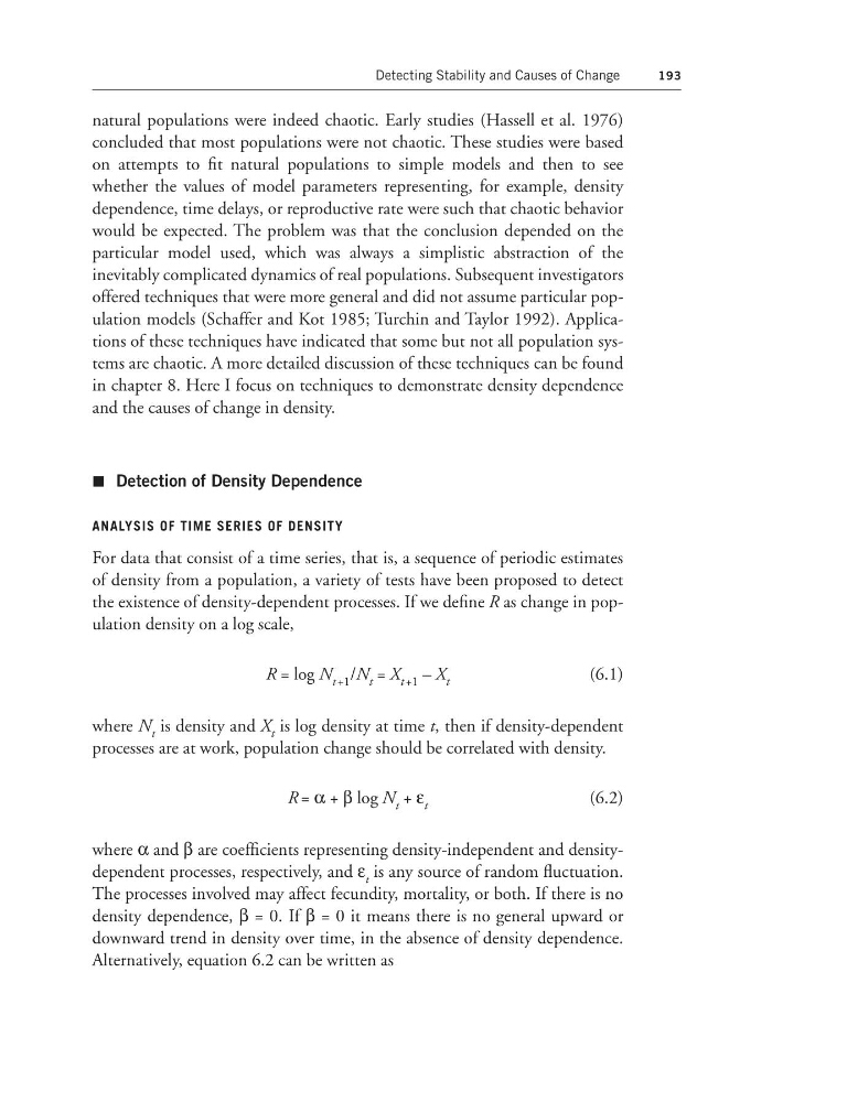
the existence of density-dependent processes. If we define R as change in population density on a log scale,
R = log N t +1 /N t = X t +1 – X t
(6.1)
where N t is density and X t is log density at time t, then if density-dependent
processes are at work, population change should be correlated with density.
R = α + β log N t + ε t
(6.2)
where α and β are coefficients representing density-independent and densitydependent processes, respectively, and ε t is any source of random fluctuation.
The processes involved may affect fecundity, mortality, or both. If there is no
density dependence, β = 0. If β = 0 it means there is no general upward or
downward trend in density over time, in the absence of density dependence.
Alternatively, equation 6.2 can be written as
193
natural populations were indeed chaotic. Early studies (Hassell et al. 1976)
concluded that most populations were not chaotic. These studies were based
on attempts to fit natural populations to simple models and then to see
whether the values of model parameters representing, for example, density
dependence, time delays, or reproductive rate were such that chaotic behavior
would be expected. The problem was that the conclusion depended on the
particular model used, which was always a simplistic abstraction of the
inevitably complicated dynamics of real populations. Subsequent investigators
offered techniques that were more general and did not assume particular population models (Schaffer and Kot 1985; Turchin and Taylor 1992). Applications of these techniques have indicated that some but not all population systems are chaotic. A more detailed discussion of these techniques can be found
in chapter 8. Here I focus on techniques to demonstrate density dependence
and the causes of change in density.
Detection of Density Dependence
ANALYSIS OF TIME SERIES OF DENSITY
For data that consist of a time series, that is, a sequence of periodic estimates
of density from a population, a variety of tests have been proposed to detect
the existence of density-dependent processes. If we define R as change in population density on a log scale,
R = log N t +1 /N t = X t +1 – X t
(6.1)
where N t is density and X t is log density at time t, then if density-dependent
processes are at work, population change should be correlated with density.
R = α + β log N t + ε t
(6.2)
where α and β are coefficients representing density-independent and densitydependent processes, respectively, and ε t is any source of random fluctuation.
The processes involved may affect fecundity, mortality, or both. If there is no
density dependence, β = 0. If β = 0 it means there is no general upward or
downward trend in density over time, in the absence of density dependence.
Alternatively, equation 6.2 can be written as