

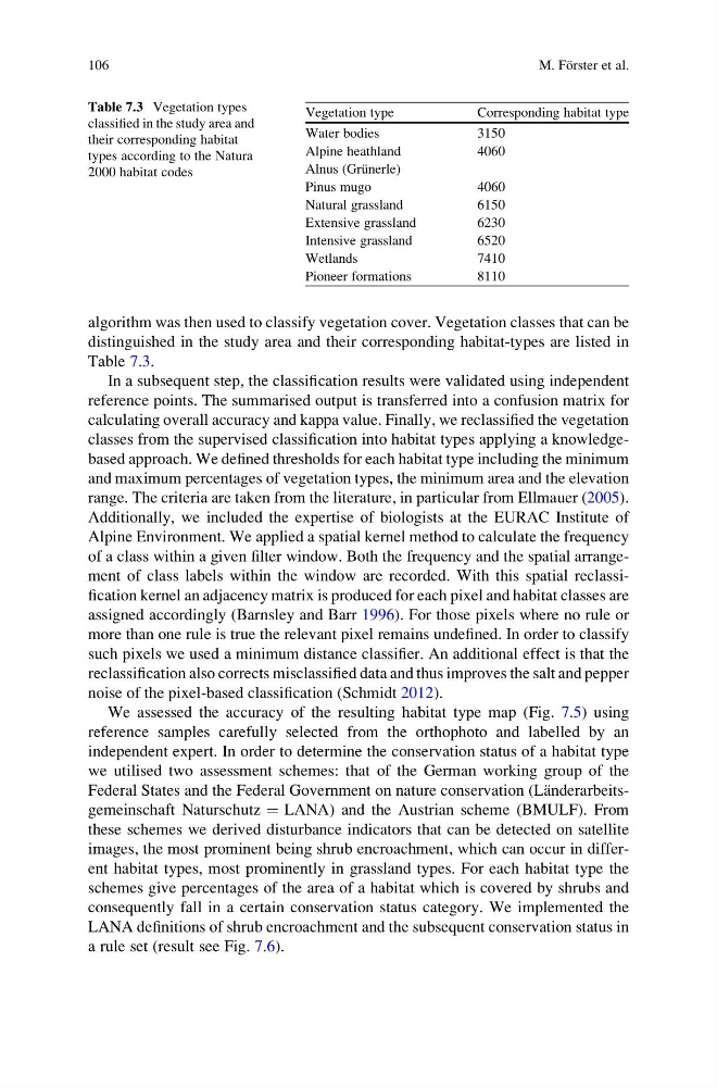
algorithm was then used to classify vegetation cover. Vegetation classes that can be
distinguished in the study area and their corresponding habitat-types are listed in
Table 7.3.
In a subsequent step, the classification results were validated using independent
reference points. The summarised output is transferred into a confusion matrix for
calculating overall accuracy and kappa value. Finally, we reclassified the vegetation
classes from the supervised classification into habitat types applying a knowledgebased approach. We defined thresholds for each habitat type including the minimum
and maximum percentages of vegetation types, the minimum area and the elevation
range. The criteria are taken from the literature, in particular from Ellmauer (2005).
Additionally, we included the expertise of biologists at the EURAC Institute of
Alpine Environment. We applied a spatial kernel method to calculate the frequency
of a class within a given filter window. Both the frequency and the spatial arrangement of class labels within the window are recorded. With this spatial reclassification kernel an adjacency matrix is produced for each pixel and habitat classes are
assigned accordingly (Barnsley and Barr 1996). For those pixels where no rule or
more than one rule is true the relevant pixel remains undefined. In order to classify
such pixels we used a minimum distance classifier. An additional effect is that the
reclassification also corrects misclassified data and thus improves the salt and pepper
noise of the pixel-based classification (Schmidt 2012).
We assessed the accuracy of the resulting habitat type map (Fig. 7.5) using
reference samples carefully selected from the orthophoto and labelled by an
independent expert. In order to determine the conservation status of a habitat type
we utilised two assessment schemes: that of the German working group of the
Federal States and the Federal Government on nature conservation (La ¨nderarbeitsgemeinschaft Naturschutz ¼ LANA) and the Austrian scheme (BMULF). From
these schemes we derived disturbance indicators that can be detected on satellite
images, the most prominent being shrub encroachment, which can occur in different habitat types, most prominently in grassland types. For each habitat type the
schemes give percentages of the area of a habitat which is covered by shrubs and
consequently fall in a certain conservation status category. We implemented the
LANA definitions of shrub encroachment and the subsequent conservation status in
a rule set (result see Fig. 7.6).
Table 7.3 Vegetation types
classified in the study area and
their corresponding habitat
types according to the Natura
2000 habitat codes
Vegetation type
Corresponding habitat type
Water bodies
3150
Alpine heathland
4060
Alnus (Gru ¨nerle)
Pinus mugo
4060
Natural grassland
6150
Extensive grassland
6230
Intensive grassland
6520
Wetlands
7410
Pioneer formations
8110
106
M. Fo ¨rster et al.
distinguished in the study area and their corresponding habitat-types are listed in
Table 7.3.
In a subsequent step, the classification results were validated using independent
reference points. The summarised output is transferred into a confusion matrix for
calculating overall accuracy and kappa value. Finally, we reclassified the vegetation
classes from the supervised classification into habitat types applying a knowledgebased approach. We defined thresholds for each habitat type including the minimum
and maximum percentages of vegetation types, the minimum area and the elevation
range. The criteria are taken from the literature, in particular from Ellmauer (2005).
Additionally, we included the expertise of biologists at the EURAC Institute of
Alpine Environment. We applied a spatial kernel method to calculate the frequency
of a class within a given filter window. Both the frequency and the spatial arrangement of class labels within the window are recorded. With this spatial reclassification kernel an adjacency matrix is produced for each pixel and habitat classes are
assigned accordingly (Barnsley and Barr 1996). For those pixels where no rule or
more than one rule is true the relevant pixel remains undefined. In order to classify
such pixels we used a minimum distance classifier. An additional effect is that the
reclassification also corrects misclassified data and thus improves the salt and pepper
noise of the pixel-based classification (Schmidt 2012).
We assessed the accuracy of the resulting habitat type map (Fig. 7.5) using
reference samples carefully selected from the orthophoto and labelled by an
independent expert. In order to determine the conservation status of a habitat type
we utilised two assessment schemes: that of the German working group of the
Federal States and the Federal Government on nature conservation (La ¨nderarbeitsgemeinschaft Naturschutz ¼ LANA) and the Austrian scheme (BMULF). From
these schemes we derived disturbance indicators that can be detected on satellite
images, the most prominent being shrub encroachment, which can occur in different habitat types, most prominently in grassland types. For each habitat type the
schemes give percentages of the area of a habitat which is covered by shrubs and
consequently fall in a certain conservation status category. We implemented the
LANA definitions of shrub encroachment and the subsequent conservation status in
a rule set (result see Fig. 7.6).
Table 7.3 Vegetation types
classified in the study area and
their corresponding habitat
types according to the Natura
2000 habitat codes
Vegetation type
Corresponding habitat type
Water bodies
3150
Alpine heathland
4060
Alnus (Gru ¨nerle)
Pinus mugo
4060
Natural grassland
6150
Extensive grassland
6230
Intensive grassland
6520
Wetlands
7410
Pioneer formations
8110
106
M. Fo ¨rster et al.