

414
6 Applications: Two-Region Pebble Beds
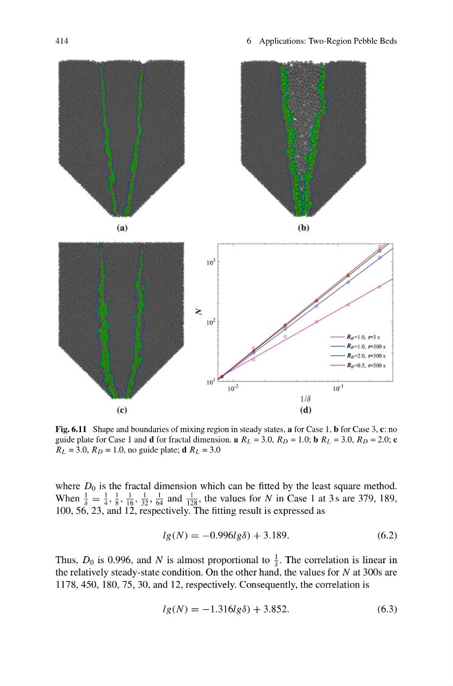
Fig. 6.11 Shape and boundaries of mixing region in steady states, a for Case 1, b for Case 3, c: no
guide plate for Case 1 and d for fractal dimension. a R L = 3.0, R D = 1.0; b R L = 3.0, R D = 2.0; c
R L = 3.0, R D = 1.0, no guide plate; d R L = 3.0
where D 0 is the fractal dimension which can be fitted by the least square method.
When
1
δ
=
1
4
,
1
8
,
1
16
,
1
32
,
1
64
and
1
128
, the values for N in Case 1 at 3 s are 379, 189,
100, 56, 23, and 12, respectively. The fitting result is expressed as
lg(N ) = −0.996lgδ) + 3.189.
(6.2)
Thus, D 0 is 0.996, and N is almost proportional to
1
δ
. The correlation is linear in
the relatively steady-state condition. On the other hand, the values for N at 300s are
1178, 450, 180, 75, 30, and 12, respectively. Consequently, the correlation is
lg(N ) = −1.316lgδ) + 3.852.
(6.3)
6 Applications: Two-Region Pebble Beds
Fig. 6.11 Shape and boundaries of mixing region in steady states, a for Case 1, b for Case 3, c: no
guide plate for Case 1 and d for fractal dimension. a R L = 3.0, R D = 1.0; b R L = 3.0, R D = 2.0; c
R L = 3.0, R D = 1.0, no guide plate; d R L = 3.0
where D 0 is the fractal dimension which can be fitted by the least square method.
When
1
δ
=
1
4
,
1
8
,
1
16
,
1
32
,
1
64
and
1
128
, the values for N in Case 1 at 3 s are 379, 189,
100, 56, 23, and 12, respectively. The fitting result is expressed as
lg(N ) = −0.996lgδ) + 3.189.
(6.2)
Thus, D 0 is 0.996, and N is almost proportional to
1
δ
. The correlation is linear in
the relatively steady-state condition. On the other hand, the values for N at 300s are
1178, 450, 180, 75, 30, and 12, respectively. Consequently, the correlation is
lg(N ) = −1.316lgδ) + 3.852.
(6.3)