

378
5 Numerical Models for Pebble-Bed Heat Transfer
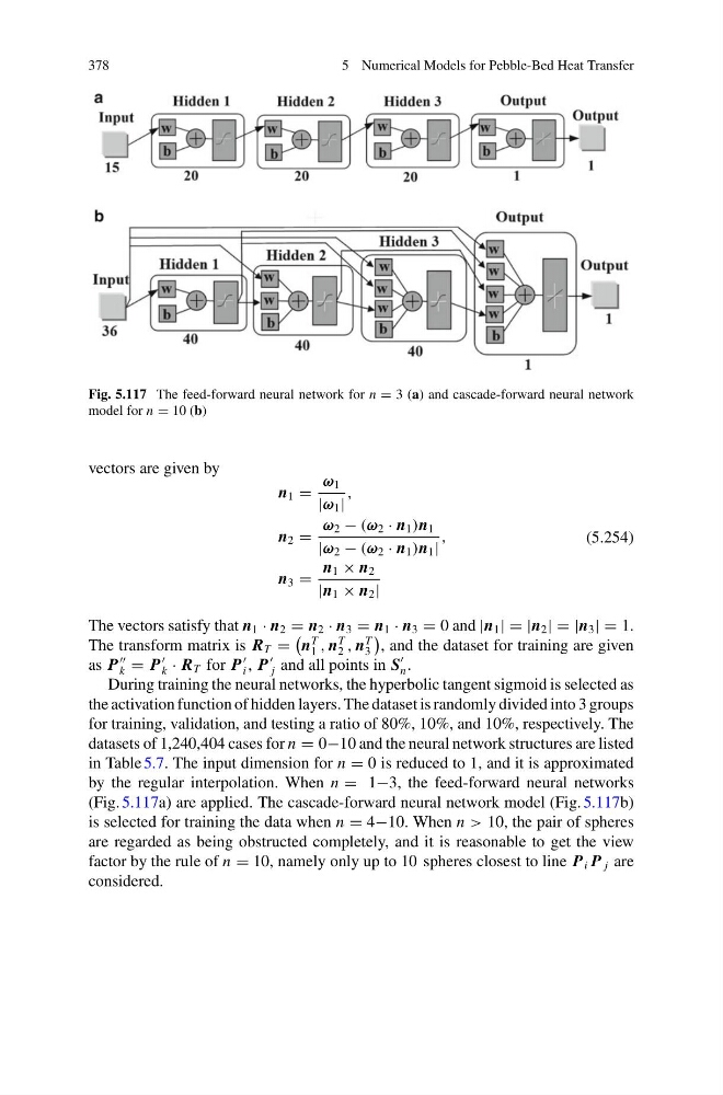
Fig. 5.117 The feed-forward neural network for n = 3 (a) and cascade-forward neural network
model for n = 10 (b)
vectors are given by
n 1 =
ω 1
|ω 1 |
,
n 2 =
ω 2 − (ω 2 · n 1 )n 1
|ω 2 − (ω 2 · n 1 )n 1 |
,
n 3 =
n 1 × n 2
|n 1 × n 2 |
(5.254)
The vectors satisfy that n 1 · n 2 = n 2 · n 3 = n 1 · n 3 = 0 and |n 1 | = |n 2 | = |n 3 | = 1.
The transform matrix is R T =
n
T
1 , n
T
2 , n
T
3
, and the dataset for training are given
as P
k = P
k · R T for P
i , P
j and all points in S
n .
During training the neural networks, the hyperbolic tangent sigmoid is selected as
the activation function of hidden layers. The dataset is randomly divided into 3 groups
for training, validation, and testing a ratio of 80%, 10%, and 10%, respectively. The
datasets of 1,240,404 cases for n = 0−10 and the neural network structures are listed
in Table 5.7. The input dimension for n = 0 is reduced to 1, and it is approximated
by the regular interpolation. When n = 1−3, the feed-forward neural networks
(Fig. 5.117a) are applied. The cascade-forward neural network model (Fig. 5.117b)
is selected for training the data when n = 4−10. When n > 10, the pair of spheres
are regarded as being obstructed completely, and it is reasonable to get the view
factor by the rule of n = 10, namely only up to 10 spheres closest to line P i P j are
considered.
5 Numerical Models for Pebble-Bed Heat Transfer
Fig. 5.117 The feed-forward neural network for n = 3 (a) and cascade-forward neural network
model for n = 10 (b)
vectors are given by
n 1 =
ω 1
|ω 1 |
,
n 2 =
ω 2 − (ω 2 · n 1 )n 1
|ω 2 − (ω 2 · n 1 )n 1 |
,
n 3 =
n 1 × n 2
|n 1 × n 2 |
(5.254)
The vectors satisfy that n 1 · n 2 = n 2 · n 3 = n 1 · n 3 = 0 and |n 1 | = |n 2 | = |n 3 | = 1.
The transform matrix is R T =
n
T
1 , n
T
2 , n
T
3
, and the dataset for training are given
as P
k = P
k · R T for P
i , P
j and all points in S
n .
During training the neural networks, the hyperbolic tangent sigmoid is selected as
the activation function of hidden layers. The dataset is randomly divided into 3 groups
for training, validation, and testing a ratio of 80%, 10%, and 10%, respectively. The
datasets of 1,240,404 cases for n = 0−10 and the neural network structures are listed
in Table 5.7. The input dimension for n = 0 is reduced to 1, and it is approximated
by the regular interpolation. When n = 1−3, the feed-forward neural networks
(Fig. 5.117a) are applied. The cascade-forward neural network model (Fig. 5.117b)
is selected for training the data when n = 4−10. When n > 10, the pair of spheres
are regarded as being obstructed completely, and it is reasonable to get the view
factor by the rule of n = 10, namely only up to 10 spheres closest to line P i P j are
considered.