

168
4 Numerical Methods and Simulation for Pebble Flows
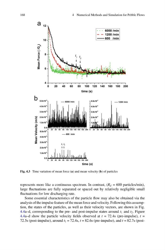
Fig. 4.3 Time variation of mean force (a) and mean velocity (b) of particles
represents more like a continuous spectrum. In contrast, (R d = 600 particles/min),
large fluctuations are fully separated or spaced out by relatively negligible small
fluctuations for low discharging rate.
Some essential characteristics of the particle flow may also be obtained via the
analysis of the impulse feature of the mean force and velocity. Following this assumption, the states of the particles, as well as their velocity vectors, are shown in Fig.
4.4a–d, corresponding to the pre- and post-impulse states around t 1 and t 2 . Figure
4.4a–d show the particle velocity fields observed at t = 72.4s (pre-impulse), t =
72.5s (post-impulse), around t 1 = 72.4s, t = 82.6s (pre-impulse), and t = 82.7s (post-
4 Numerical Methods and Simulation for Pebble Flows
Fig. 4.3 Time variation of mean force (a) and mean velocity (b) of particles
represents more like a continuous spectrum. In contrast, (R d = 600 particles/min),
large fluctuations are fully separated or spaced out by relatively negligible small
fluctuations for low discharging rate.
Some essential characteristics of the particle flow may also be obtained via the
analysis of the impulse feature of the mean force and velocity. Following this assumption, the states of the particles, as well as their velocity vectors, are shown in Fig.
4.4a–d, corresponding to the pre- and post-impulse states around t 1 and t 2 . Figure
4.4a–d show the particle velocity fields observed at t = 72.4s (pre-impulse), t =
72.5s (post-impulse), around t 1 = 72.4s, t = 82.6s (pre-impulse), and t = 82.7s (post-