

3.3 Effective Thermal Diffusivity and Conductivity
145
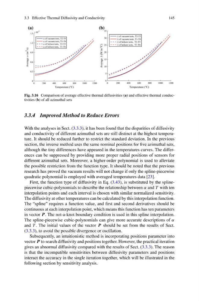
Fig. 3.16 Comparison of average effective thermal diffusivities (a) and effective thermal conductivities (b) of all azimuthal sets
3.3.4 Improved Method to Reduce Errors
With the analyses in Sect. (3.3.3), it has been found that the disparities of diffusivity
and conductivity of different azimuthal sets are still distinct at the highest temperature. It should be reduced further to restrict the standard deviation. In the previous
section, the inverse method uses the same nominal positions for five azimuthal sets,
although the tiny differences have appeared in the temperatures curves. The differences can be suppressed by providing more proper radial positions of sensors for
different azimuthal sets. Moreover, a higher-order polynomial is used to alleviate
the possible restriction from the function type. It should be noted that the previous
research has proved the vacuum results will not change if only the spline-piecewise
quadratic polynomial is employed with averaged temperatures data [23].
First, the function type of diffusivity in Eq. (3.43), is substituted by the splinepiecewise cubic-polynomials to describe the relationship between α and T with ten
interpolation points and each interval is chosen with similar normalized sensitivity.
The diffusivity at other temperatures can be calculated by this interpolation function.
The “spline” requires a function value, and first and second derivatives should be
continuous at each interpolation point, which means this function has ten parameters
in vector P. The not-a-knot boundary condition is used in this spline interpolation.
The spline-piecewise cubic-polynomials can give more accurate descriptions of α
and T . The initial values of the vector P should be set from the results of Sect.
(3.3.3), to avoid the possible divergence or oscillation.
Subsequently, an intuitionistic method is incorporating positions parameter into
vector P to search diffusivity and positions together. However, the practical iteration
gives an abnormal diffusivity compared with the results of Sect. (3.3.3). The reason
is that the incompatible sensitivities between diffusivity parameters and positions
interact the accuracy in the single iteration together, which will be illustrated in the
following section by sensitivity analysis.
145
Fig. 3.16 Comparison of average effective thermal diffusivities (a) and effective thermal conductivities (b) of all azimuthal sets
3.3.4 Improved Method to Reduce Errors
With the analyses in Sect. (3.3.3), it has been found that the disparities of diffusivity
and conductivity of different azimuthal sets are still distinct at the highest temperature. It should be reduced further to restrict the standard deviation. In the previous
section, the inverse method uses the same nominal positions for five azimuthal sets,
although the tiny differences have appeared in the temperatures curves. The differences can be suppressed by providing more proper radial positions of sensors for
different azimuthal sets. Moreover, a higher-order polynomial is used to alleviate
the possible restriction from the function type. It should be noted that the previous
research has proved the vacuum results will not change if only the spline-piecewise
quadratic polynomial is employed with averaged temperatures data [23].
First, the function type of diffusivity in Eq. (3.43), is substituted by the splinepiecewise cubic-polynomials to describe the relationship between α and T with ten
interpolation points and each interval is chosen with similar normalized sensitivity.
The diffusivity at other temperatures can be calculated by this interpolation function.
The “spline” requires a function value, and first and second derivatives should be
continuous at each interpolation point, which means this function has ten parameters
in vector P. The not-a-knot boundary condition is used in this spline interpolation.
The spline-piecewise cubic-polynomials can give more accurate descriptions of α
and T . The initial values of the vector P should be set from the results of Sect.
(3.3.3), to avoid the possible divergence or oscillation.
Subsequently, an intuitionistic method is incorporating positions parameter into
vector P to search diffusivity and positions together. However, the practical iteration
gives an abnormal diffusivity compared with the results of Sect. (3.3.3). The reason
is that the incompatible sensitivities between diffusivity parameters and positions
interact the accuracy in the single iteration together, which will be illustrated in the
following section by sensitivity analysis.