

3.3 Effective Thermal Diffusivity and Conductivity
137
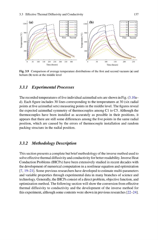
Fig. 3.9 Comparison of average temperature distributions of the first and second vacuum (a) and
helium (b) tests at the middle level
3.3.1 Experimental Processes
The recorded temperatures of five individual azimuthal sets are shown in Fig. (3.10a–
d). Each figure includes 30 lines corresponding to the temperatures at 30 (six radial
points at five azimuthal sets) measuring points in the middle level. The figures reveal
the expected azimuthal symmetry of thermocouples among C1 to C5. Although the
thermocouples have been installed as accurately as possible in their positions, it
appears that there are still some differences among the five points in the same radial
position, which are caused by the errors of thermocouple installation and random
packing structure in the radial position.
3.3.2 Methodology Description
This section presents a complete but brief methodology of the inverse method used to
solve effective thermal diffusivity and conductivity for better readability. Inverse Heat
Conduction Problems (IHCPs) have been extensively studied in recent decades with
the development of numerical computation in a nonlinear equation and optimization
[7, 19–21]. Some previous researchers have developed to estimate multi-parameters
and variable properties through experimental data in many branches of science and
technology. Generally, the IHCPs consist of a direct problem, objective function, and
optimization method. The following section will show the conversion from effective
thermal diffusivity to conductivity and the development of the inverse method for
this experiment, although some contents were shown in previous researches [22–24].
137
Fig. 3.9 Comparison of average temperature distributions of the first and second vacuum (a) and
helium (b) tests at the middle level
3.3.1 Experimental Processes
The recorded temperatures of five individual azimuthal sets are shown in Fig. (3.10a–
d). Each figure includes 30 lines corresponding to the temperatures at 30 (six radial
points at five azimuthal sets) measuring points in the middle level. The figures reveal
the expected azimuthal symmetry of thermocouples among C1 to C5. Although the
thermocouples have been installed as accurately as possible in their positions, it
appears that there are still some differences among the five points in the same radial
position, which are caused by the errors of thermocouple installation and random
packing structure in the radial position.
3.3.2 Methodology Description
This section presents a complete but brief methodology of the inverse method used to
solve effective thermal diffusivity and conductivity for better readability. Inverse Heat
Conduction Problems (IHCPs) have been extensively studied in recent decades with
the development of numerical computation in a nonlinear equation and optimization
[7, 19–21]. Some previous researchers have developed to estimate multi-parameters
and variable properties through experimental data in many branches of science and
technology. Generally, the IHCPs consist of a direct problem, objective function, and
optimization method. The following section will show the conversion from effective
thermal diffusivity to conductivity and the development of the inverse method for
this experiment, although some contents were shown in previous researches [22–24].