

126
3 Experiments in Pebble Bed Heat Transfer
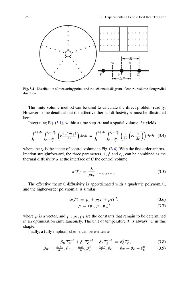
Fig. 3.4 Distribution of measuring points and the schematic diagram of control volume along radial
direction
The finite volume method can be used to calculate the direct problem readily.
However, some details about the effective thermal diffusivity α must be illustrated
here.
Integrating Eq. (3.1), within a time step Δt and a spatial volume Δr yields
t+Δt
t
r c +
Δr
2
r c −
Δr
2
r
∂(T ¯
ρc g )
∂t
drdt =
t+Δt
t
r c +
Δr
2
r c −
Δr
2
∂
∂r
r λ
∂ T
∂r
drdt, (3.4)
where the r c is the center of control volume in Fig. (3.4). With the first order approximation straightforward, the three parameters, λ, ¯
ρ and c g , can be combined as the
thermal diffusivity α at the interface of C the control volume.
α(T ) =
λ
¯
ρc g
r = e, or r = w
(3.5)
The effective thermal diffusivity is approximated with a quadratic polynomial,
and the higher-order polynomial is similar
α(T ) = p 1 + p 2 T + p 3 T
2
,
(3.6)
p = ( p 1 , p 2 , p 3 )
T
(3.7)
where p is a vector, and p 1 , p 2 , p 3 are the constants that remain to be determined
in an optimization simultaneously. The unit of temperature T is always
◦ C in this
chapter.
finally, a fully implicit scheme can be written as
−β W T
n+1
W
+ β C T
n+1
C
− β E T
n+1
E
= β
0
C T
n
C ,
(3.8)
β W =
α w r w
δr
, β E =
α e r e
δr
, β
0
C =
r c Δr
Δt
, β C = β W + β E + β
0
C
(3.9)
3 Experiments in Pebble Bed Heat Transfer
Fig. 3.4 Distribution of measuring points and the schematic diagram of control volume along radial
direction
The finite volume method can be used to calculate the direct problem readily.
However, some details about the effective thermal diffusivity α must be illustrated
here.
Integrating Eq. (3.1), within a time step Δt and a spatial volume Δr yields
t+Δt
t
r c +
Δr
2
r c −
Δr
2
r
∂(T ¯
ρc g )
∂t
drdt =
t+Δt
t
r c +
Δr
2
r c −
Δr
2
∂
∂r
r λ
∂ T
∂r
drdt, (3.4)
where the r c is the center of control volume in Fig. (3.4). With the first order approximation straightforward, the three parameters, λ, ¯
ρ and c g , can be combined as the
thermal diffusivity α at the interface of C the control volume.
α(T ) =
λ
¯
ρc g
r = e, or r = w
(3.5)
The effective thermal diffusivity is approximated with a quadratic polynomial,
and the higher-order polynomial is similar
α(T ) = p 1 + p 2 T + p 3 T
2
,
(3.6)
p = ( p 1 , p 2 , p 3 )
T
(3.7)
where p is a vector, and p 1 , p 2 , p 3 are the constants that remain to be determined
in an optimization simultaneously. The unit of temperature T is always
◦ C in this
chapter.
finally, a fully implicit scheme can be written as
−β W T
n+1
W
+ β C T
n+1
C
− β E T
n+1
E
= β
0
C T
n
C ,
(3.8)
β W =
α w r w
δr
, β E =
α e r e
δr
, β
0
C =
r c Δr
Δt
, β C = β W + β E + β
0
C
(3.9)