

2.5 Particle Velocimetry Measurements
95
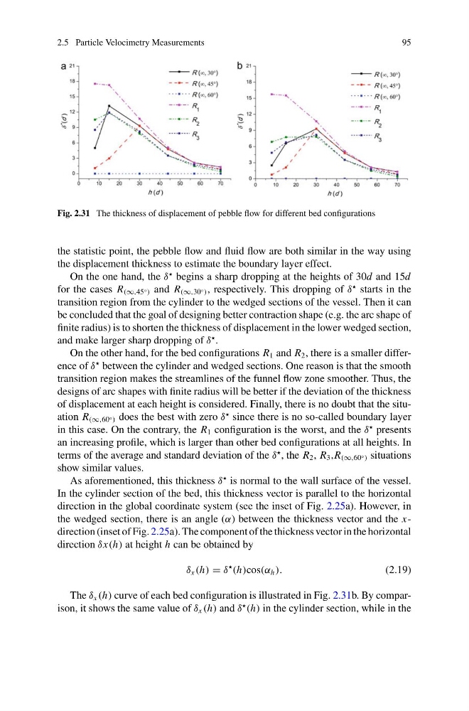
Fig. 2.31 The thickness of displacement of pebble flow for different bed configurations
the statistic point, the pebble flow and fluid flow are both similar in the way using
the displacement thickness to estimate the boundary layer effect.
On the one hand, the δ
begins a sharp dropping at the heights of 30d and 15d
for the cases R (∞,45 ◦ ) and R (∞,30 ◦ ) , respectively. This dropping of δ
starts in the
transition region from the cylinder to the wedged sections of the vessel. Then it can
be concluded that the goal of designing better contraction shape (e.g. the arc shape of
finite radius) is to shorten the thickness of displacement in the lower wedged section,
and make larger sharp dropping of δ
.
On the other hand, for the bed configurations R 1 and R 2 , there is a smaller difference of δ
between the cylinder and wedged sections. One reason is that the smooth
transition region makes the streamlines of the funnel flow zone smoother. Thus, the
designs of arc shapes with finite radius will be better if the deviation of the thickness
of displacement at each height is considered. Finally, there is no doubt that the situation R (∞,60 ◦ ) does the best with zero δ
since there is no so-called boundary layer
in this case. On the contrary, the R 1 configuration is the worst, and the δ
presents
an increasing profile, which is larger than other bed configurations at all heights. In
terms of the average and standard deviation of the δ
, the R 2 , R 3 ,R (∞,60 ◦ ) situations
show similar values.
As aforementioned, this thickness δ
is normal to the wall surface of the vessel.
In the cylinder section of the bed, this thickness vector is parallel to the horizontal
direction in the global coordinate system (see the inset of Fig. 2.25a). However, in
the wedged section, there is an angle (α) between the thickness vector and the xdirection (inset of Fig. 2.25a). The component of the thickness vector in the horizontal
direction δx(h) at height h can be obtained by
δ x (h) = δ
(h)cos(α h ).
(2.19)
The δ x (h) curve of each bed configuration is illustrated in Fig. 2.31b. By comparison, it shows the same value of δ x (h) and δ
(h) in the cylinder section, while in the
95
Fig. 2.31 The thickness of displacement of pebble flow for different bed configurations
the statistic point, the pebble flow and fluid flow are both similar in the way using
the displacement thickness to estimate the boundary layer effect.
On the one hand, the δ
begins a sharp dropping at the heights of 30d and 15d
for the cases R (∞,45 ◦ ) and R (∞,30 ◦ ) , respectively. This dropping of δ
starts in the
transition region from the cylinder to the wedged sections of the vessel. Then it can
be concluded that the goal of designing better contraction shape (e.g. the arc shape of
finite radius) is to shorten the thickness of displacement in the lower wedged section,
and make larger sharp dropping of δ
.
On the other hand, for the bed configurations R 1 and R 2 , there is a smaller difference of δ
between the cylinder and wedged sections. One reason is that the smooth
transition region makes the streamlines of the funnel flow zone smoother. Thus, the
designs of arc shapes with finite radius will be better if the deviation of the thickness
of displacement at each height is considered. Finally, there is no doubt that the situation R (∞,60 ◦ ) does the best with zero δ
since there is no so-called boundary layer
in this case. On the contrary, the R 1 configuration is the worst, and the δ
presents
an increasing profile, which is larger than other bed configurations at all heights. In
terms of the average and standard deviation of the δ
, the R 2 , R 3 ,R (∞,60 ◦ ) situations
show similar values.
As aforementioned, this thickness δ
is normal to the wall surface of the vessel.
In the cylinder section of the bed, this thickness vector is parallel to the horizontal
direction in the global coordinate system (see the inset of Fig. 2.25a). However, in
the wedged section, there is an angle (α) between the thickness vector and the xdirection (inset of Fig. 2.25a). The component of the thickness vector in the horizontal
direction δx(h) at height h can be obtained by
δ x (h) = δ
(h)cos(α h ).
(2.19)
The δ x (h) curve of each bed configuration is illustrated in Fig. 2.31b. By comparison, it shows the same value of δ x (h) and δ
(h) in the cylinder section, while in the