

3.1 Density Matrix
49
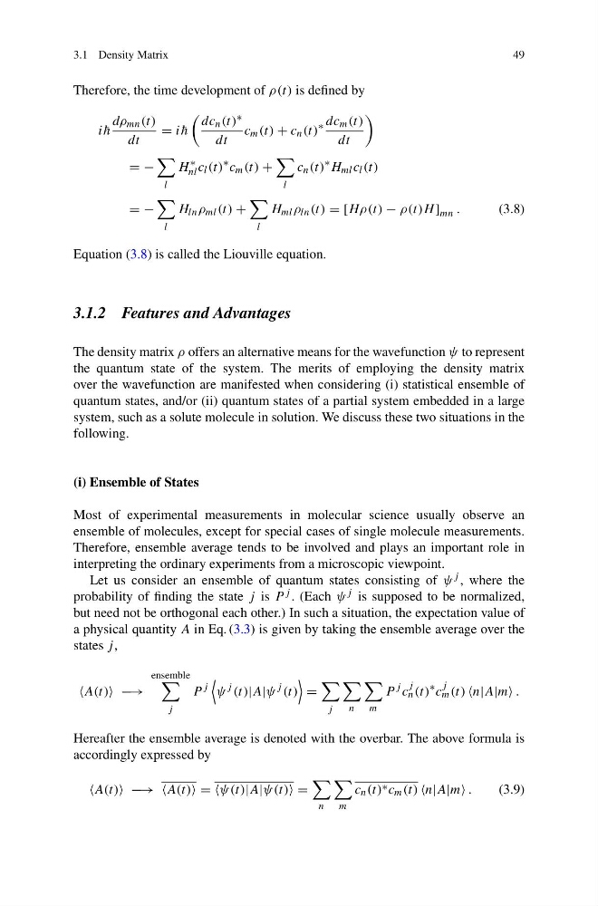
Therefore, the time development of ρ(t) is defined by
i ¯
h
dρ mn (t)
dt
= i ¯
h
dc n (t) ∗
dt
c m (t) + c n (t)
∗ dc m (t)
dt
= −
l
H
∗
nl c l (t)
∗ c m (t) +
l
c n (t)
∗ H ml c l (t)
= −
l
H ln ρ ml (t) +
l
H ml ρ ln (t) = [Hρ(t) − ρ(t)H ] mn .
(3.8)
Equation (3.8) is called the Liouville equation.
3.1.2 Features and Advantages
The density matrix ρ offers an alternative means for the wavefunction ψ to represent
the quantum state of the system. The merits of employing the density matrix
over the wavefunction are manifested when considering (i) statistical ensemble of
quantum states, and/or (ii) quantum states of a partial system embedded in a large
system, such as a solute molecule in solution. We discuss these two situations in the
following.
(i) Ensemble of States
Most of experimental measurements in molecular science usually observe an
ensemble of molecules, except for special cases of single molecule measurements.
Therefore, ensemble average tends to be involved and plays an important role in
interpreting the ordinary experiments from a microscopic viewpoint.
Let us consider an ensemble of quantum states consisting of ψ j , where the
probability of finding the state j is P j . (Each ψ j is supposed to be normalized,
but need not be orthogonal each other.) In such a situation, the expectation value of
a physical quantity A in Eq. (3.3) is given by taking the ensemble average over the
states j ,
A(t) − −→
ensemble
j
P
j
ψ
j (t)|A|ψ
j (t)
=
j
n
m
P
j c
j
n (t)
∗ c
j
m (t) n|A|m .
Hereafter the ensemble average is denoted with the overbar. The above formula is
accordingly expressed by
A(t) − −→ A(t) = ψ(t)|A|ψ(t) =
n
m
c n (t) ∗ c m (t) n|A|m .
(3.9)
49
Therefore, the time development of ρ(t) is defined by
i ¯
h
dρ mn (t)
dt
= i ¯
h
dc n (t) ∗
dt
c m (t) + c n (t)
∗ dc m (t)
dt
= −
l
H
∗
nl c l (t)
∗ c m (t) +
l
c n (t)
∗ H ml c l (t)
= −
l
H ln ρ ml (t) +
l
H ml ρ ln (t) = [Hρ(t) − ρ(t)H ] mn .
(3.8)
Equation (3.8) is called the Liouville equation.
3.1.2 Features and Advantages
The density matrix ρ offers an alternative means for the wavefunction ψ to represent
the quantum state of the system. The merits of employing the density matrix
over the wavefunction are manifested when considering (i) statistical ensemble of
quantum states, and/or (ii) quantum states of a partial system embedded in a large
system, such as a solute molecule in solution. We discuss these two situations in the
following.
(i) Ensemble of States
Most of experimental measurements in molecular science usually observe an
ensemble of molecules, except for special cases of single molecule measurements.
Therefore, ensemble average tends to be involved and plays an important role in
interpreting the ordinary experiments from a microscopic viewpoint.
Let us consider an ensemble of quantum states consisting of ψ j , where the
probability of finding the state j is P j . (Each ψ j is supposed to be normalized,
but need not be orthogonal each other.) In such a situation, the expectation value of
a physical quantity A in Eq. (3.3) is given by taking the ensemble average over the
states j ,
A(t) − −→
ensemble
j
P
j
ψ
j (t)|A|ψ
j (t)
=
j
n
m
P
j c
j
n (t)
∗ c
j
m (t) n|A|m .
Hereafter the ensemble average is denoted with the overbar. The above formula is
accordingly expressed by
A(t) − −→ A(t) = ψ(t)|A|ψ(t) =
n
m
c n (t) ∗ c m (t) n|A|m .
(3.9)